Monthly Archives: March 2014

On Sensible Units for Spectra

How do you express a spectrum in a universal way, without appealing to units?

Spectra are fundamental to astronomy.  When we disperse light from stars, we are mathematically taking the power spectrum of the electric field as a function of time, but physically we are sorting the light by energy/wavelength/wavenumber/frequency/color, i.e. making a rainbow out of it.  Some colors are better represented than others:  the quantification of this observation is the spectrum.  Why do we need units for this?

Astronomers have lots of funny names and units for the spectrum.  If your spectrum is very coarse then you might call it a spectral energy distribution (SED), or just refer to the “broadband photometry” or “N-band magnitude” of the object (where N is some filter).  If you are just looking at whether redder or bluer photons are more common you might refer to its spectral index (especially in the high- and low-energy regimes).  If you have a very narrow-band or high resolution spectra of an absorption or emission line you might just refer to a “line profile”.  

But it’s units where we get really creative.  The fundamental unit of radiation is intensity, or specific surface brightness.  It measures the energy of a given color per unit time (power) coming from (or going into) some patch of sky as it crosses some surface.  It might be the upward-going intensity off of the surface of the Sun, or the downward-going intensity striking a telescope primary mirror from a patch on the moon.  Units are W/m2/sr/Hz or W/m2/sr/cm (with the last bit depending on whether you like to divide your light up by frequency or wavelength).

Astronomers, being astronomers, are not content to just use one set of units.  We use cgs versions, we multiply by big numbers from there (Janskys), we use brightness temperature (so Kelvins is a unit of intensity!) we express wavelength differences as velocities (so Kelvin kilometers per second (K k/s) is a flux!) we count photons instead of ergs, and so on.  And of course we love to take the base ten logarithm and multiply by 2.5, make it go backwards, and call it a “magnitude” (for back-compatibility with naked-eye Greek astronomers, of course).

What’s more, the whole “surface brightness”/”per patch of sky” thing is generally glossed over in favor of just measuring “flux”, the total amount of energy collected per area per second (something David Hogg disapproves of, and he has a good point).  Flux has units of W/m2.

If you disperse the light you collect, then you have to specify how big your color/frequency/energy/wavelength/wavenumber bins are to express your spectrum in physical units.  We call this a specific flux or flux density or spectral irradiance, and the units are W/m2/Hz or W/m2/cm or W/m2/eV or W/m2/Å (or W/m2/Gyr-1, I suppose).  If all you are doing is choosing between units of wavelength (cm vs. Å), then these units differ by just a constant factor, but switching to energy changes the underlying shape of the spectrum, which is annoying to deal with (as students calculating the Wien peak of the Planck function the world over have discovered).  This is because your bins are bigger for bluer photons if you use energy, but smaller if you use wavelength.  When you have uneven bin sizes, your histogram gets distorted.

This unfortunate situation is one reason that astronomers often publish spectra with νFν or λFλ for their units of flux density:  by multiplying the flux density by the wavelength (λ) or frequency (ν), they recover units of flux and become agnostic to the (arbitrary) choice of wavelength vs. frequency binning.  In fact, since λFλ = νFν, you can even switch between them in a paper (I’ve been guilty of this).  

Richard Wade pointed me to an interesting paper in Observatory, here, by Disney and Sparks called “On Sensible Units for Apparent Flux” published in 1982.  It begins: 

Gentlemen, —

The day must surely come when the present Babel of units to describe the apparent fluxes of astronomical objects is replaced by a more rational system….

…we feel that the sooner astronomers openly debate amongst themselves what they want the sooner action is likely to come.  Without laying claim to any originality but in the hope of stimulating such a discussion, we suggest a unit which we have presumptuously named the Hershel.

We will pause to *sigh* about he whole “gentlemen” thing and acknowledge that “ladies” (and all other astronomers) might also be interested in their discourse.

OK, moving on, Disney and Sparks go on to suggest the astronomers adopt the measure of apparent luminosity, the brilliance, B(x).  As a function, B(x) accepts as an argument the base 10 log of the frequency in Hz and returns λFλ = νFν .  Its units are Herschels, such that a source emitting one bolometric Solar luminosity per decade of frequency centered at x from a distance of 1 parsec from Earth delivers 1 Herschel of brilliance.  They define the base 10 log of the brilliance measured in Herschels to be the strength of the signal.

Screen Shot 2014-03-10 at 7.43.55 AM.png

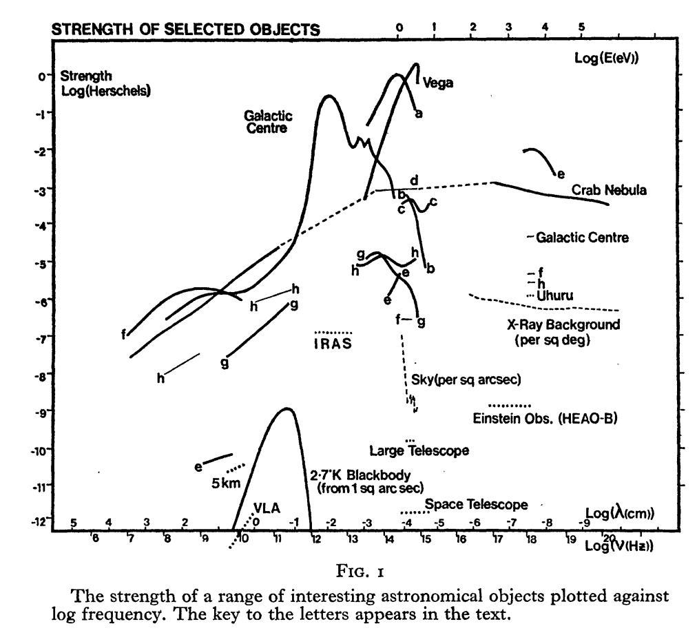
(Above, a figure from Disney and Sparks, which confusingly and unnecessarily plots intensities with a variety of scaling factors, after arguing that we need a more uniform system!)

Now, I would quibble with their choices of parsecs, Solar bolometric luminosities, and base-10 logarithms (as they said folk would).  I don’t see what’s wrong with SI (or cgs) units and natural logs (does that make me a Jansky fan?).  But I appreciate the effort.

OK, with that table-setting out of the way, let me contribute to the discussion Disney and Sparks sought to have.

In a recent paper I wanted to express the spectrum of a galaxy as a composite of many underlying sources — dust, stars, nonthermal emission, and so on — each responsible for some fraction of the total luminosity, L.  But I didn’t want to wed myself to any particular set of units — I just wanted to express the shape of the spectrum gosh darn it.  

Plots of theoretical spectra often have something like “νFν (arbitrary units)” on the y-axis; the pedant in me says that the units of flux are not arbitrary and if you want to plot a dimensionless quantity you should just do it.  I also wanted to parameterize away the distance and luminosity as a “nuisance” term, so I wrote down:

f = νFν(4πd2/L)

and called f the “dimensionless SED” of the object, or its “dimensionless spectrum”.  It’s nice because it’s area normalized to 1, so can be equally well applied to the flux or the intensity, and has no preference for things like bases of logarithms (except the natural one, I guess).  To plot it you still have to choose units for your x-axis, but that is unavoidable.

I like this because it conforms to our intuitive sense of what a “spectrum” is: a shape, without any appeal to arbitrary choices of units.  For instance, lasers emit (close to) delta functions, which need no normalization expressed as a dimensionless SED because they are also area-normalized to 1 (in physics, anyway).  

Now, you can’t use this to express how bright an object is, but for that you can use Herschels, which simply scale the dimensionless spectrum by the apparent brightness (though I think I would prefer something like Jy Hz).

What do folks think?  Useful?  Interesting, at least?  Too obvious to even write about?  Am I missing existing jargon for the “dimensionless spectrum” of an object?

55 Cancri: It’s Tricky!

As a kid I found my parents’ old LP’s: The Rolling Stones (Let It Bleed!), Bob Dylan (Blood on the Tracks!), Big Brother and the Holding Company (Cheap Thrills!).  As a result, I feel I have a good appreciation for the roots of modern rock and roll.

So it’s good to see that the kids these days are acknowledging the classics.  New Penn State grad student Ben Nelson, working with Eric Ford, has been, as he put it “remastering the RV classics” by reanalyzing the LONG data streams of radial velocities for some of the longest-known and best-observed systems, like 55 Cancri (5 planets, one transiting) and GJ 876 (4 planets, probably, with strong mean-motion resonances).

My quick and usually-good-enough approach to fitting multiplanet systems measured with multiple telescopes is to use the RVLIN approach I developed with Andrew Howard (published here, code available here, parameter uncertainties available thanks to Sharon Wang’s work here).  But this approach does not incorporate planet-planet interactions (usually not a problem — they are too small to detect for almost all systems) and is a strictly “frequentist” chi-squared approach, which is decidedly out of fashion in astronomy these days.

Ben, as any good Eric Ford grad student will, brings to the problem a rigorous Bayesian (Markov chain Monte Carlo, or “MCMC”) approach that generates parameter posteriors.  He also incorporates dynamical effects, so that planet-planet interactions are not just accounted for but can help constrain the physical parameters of the system.  His code also naturally accounts for the independent radial velocity time series not just for the four telescopes that have observed these exoplanetary systems, but for potential offsets between data streams for different detectors on the same telescope.  It also independently determines the quality of the data (the “instrumental jitter”) for each detector/telescope.

Oh, and he also incorporates dynamical stability constraints, so that long term (108 years) unstable configurations are not part of the final posterior sample.

Oh, and he does the whole thing on a supercomputer with multithreading.

Oh, and the “supercomputer” in question is actually a cluster of graphics processor units (GPU’s), which are cheap and fast but much trickier to hack into doing this sort of calculation than a “proper” supercomputer.

Really, the whole thing is a tour-de-force of how to do the problem “right”.  

Ben is also an old-school hip hop fan.  Apparently, the coincidence of the initials of Markov Chain, Monte Carlo, and “Master of Ceremonies” has been too much to resist in astronomy. First we had “emcee: The MCMC HAMMER” (http://arxiv.org/abs/1202.3665), public code by Daniel Foreman-Mackey that samples MCMC ensembles very cleverly.

Ben’s code is called RUN-DMC, for “Radial velocity Using N-body Differential evolution markov chain Monte Carlo.

Ben’s paper on the 55 Cnc system is here:http://arxiv.org/abs/1311.5229

Applying RUN-DMC to 55 Cnc, Ben finds that each planet has something interesting to teach us:

  • b and c are near a mean motion resonance, but not actually in the 3:1 resonance.  They may, however, be apsidally locked at 180 degrees with a large libration amplitude (something Eugene Chiang refers to as the “metronome” formulation of the simple harmonic oscillator problem, as opposed to the usual “pendulum” formulation about 0 degrees).  Note that the period ratio incorporating planet-planet interactions (blue) differs by many sigma from the purely Keplerian solution (orange).  (The green solutions are osculating elements, I think — you have have to average over large time intervals to determine a robust period ratio, which gives you the blue cloud).
Screen Shot 2014-03-09 at 10.39.29 AM.png

  • d’s revised period and eccentricity make it one of the best Jupiter analogs known (though it has inner massive planets, so 55 Cnc is not a good Solar System analog).  For reference, Jupiter has P=4332 and e=0.05.

Screen Shot 2014-03-09 at 10.39.13 AM.png

  • The transiting, e component is probably reasonably well aligned with the other 4 planets (within 60 degrees, based on dynamical stability), and has a density of 5.5 (+1.3/-1.0) g/cc, very close to Earth’s (5.5, though the mass of e is at least 8 times higher than Earth’s, so it probably has more volatiles and maybe a big atmosphere).
  • f is in the Habitable Zone, but its amplitude is still to low to get a good handle on its eccentricity.

Incidentally, when Ben gave a talk in our department about this code, several of our department’s freshmen were in attendance as part of an assignment in my First Year Seminar class to attend a department talk.  They said they were confused, in particular why everyone else laughed when Ben announced the name of the code was RUN-DMC.  They had never heard that term before.

Now that makes me feel old.  Run was the King of Rock!  There is none higher!  They’re in the Rock and Roll Hall of Fame for goodness’ sake!  

Kids just don’t know their history any more.

(Though as much as I, as a classic rock fan, appreciated RUN-DMC’s crossover hit Walk this Way, especially Stephen Tyler’s Kool-Aid Man burst through the wall in the video, my Seattle roots make me partial to Mix — his posse’s on Broadway.)

[Update: Be sure to keep track of Ben’s own explanation of the paper on his blog!]

The Amazing Cultural Force that is Groundhog Day

Back when I was a graduate student at Berkeley, I hosted the astronomy department Movie Night, which included sending teasers of movies we would screen in the department.  I had a lot of fun with these, but one of my favorites was the one I did for Groundhog Day. I wrote it up here, slightly revised, in 2014 in honor of Harold Ramis, who died that year.

Q:How much wood would a woodchuck chuck if a woodchuck would chuck wood?

A:Just as much wood as a woodchuck could chuck if a woodchuck would chuck wood.

I post this insight to illuminate one of the many fascinating corners of the cultural phenomenon that is Groundhog Day. Before I explain, let’s lay some groundwork.

Before the arrival of Christianity in parts Europe, many pagan cultures based their annual celebrations on agricultural events associated with the seasons. The most important of these events was often the celebration of the vernal equinox, a rebirth ceremony marking the arrival of baby crops and animals after winter. The other “quarter days”, the autumnal equinox and the winter and summer solstices, were also marked and celebrated (not just by Europeans, but by cultures around the world). Perhaps the most famous example of this practice stands today in the ruins of Stonehenge where the alignment of the stones marks the position of the setting sun on the quarter days. Likewise, the ruins of Tulum in Cozumel, Mexico feature long holes in the stone which, (just like in Indiana Jones and the Raiders of the Lost Ark) allow sunlight to illuminate a chamber only on one of the quarter days.

In addition to these holidays, cross-quarter days celebrated the days midway between quarter days. Perhaps the most famous relic of the pagan cross-quarter days in Halloween, whose imagery is still totally divorced from the Christian holiday (the Eve of the Feast of All Saints or “All Hallow’s Eve’n”), that attempted to supplant it. You see, the Roman Catholic Church, as it spread across Europe, associated many Christian holidays with these quarter and cross-quarter holidays in an attempt to ease pagans into the faith. Thus, Saturnalia and Yuletide became Christmas, the vernal equinox celebrations (complete with those images of fertility, rabbits and eggs) became Easter, All Saint’s Day supplanted the precursors to Halloween, and the 2nd of February, midway between the winter solstice and vernal equinox, became Candlemas.

Candlemas, or the Purification of the Blessed Virgin, marks the 40th day after the birth of Christ and the day, under Mosaic law, that Mary went to the temple to be purified after the birth of a son.  The pagan traditions and symbolism remained, however, as Candlemas offered a convenient marker than spring was six weeks away. Scottish tradition held that the weather on this day foretold whether spring would come early or late that year:

If Candlemas day be dry and fair,
The half o’ winter to come and mair,
If Candlemas day be wet and foul,
The half of winter’s gone at Yule.

I guess it rhymes in a Scottish accent.

Anyway, tradition holds that Roman legions brought this rule of thumb to the Germans, who associated it with the hedgehog and its shadow (since if shadows were cast on that day then “Candlemas day be dry and fair” and winter is only halfway over).  From there, the Pennsylvania Dutch (as in “Deutsch”, not as in Holland) brought the tradition to the New World, but were frustrated by the lack of hedgehogs here. To compensate, they pinned the predictive power on the local equivalent, the woodchuck (or “groundhog”).

To this day, the Punxsutawney Groundhog Club of Punxsutawney, PA promotes their local woodchuck, Phil, and every 2nd of February gathers around him as he emerges from is hole with television crews which record the event for filler segments on news broadcasts across the country.groundhog-day-driving-300x206.jpgThen in 1993, Harold Ramis overthrew thousands of years of reverent tradition with  “Groundhog Day”, a film about a weatherman, who, disgruntled at being upstaged and out-predicted by Punxsutawney Phil, is damned by the gods to repeat his day of shame until he learns the true meaning of love and, I guess, Groundhog Day.

As a result, a popular reference to Groundhog Day is now more likely to refer to a repetitive daily routine or eerie repeat of a previous experience than to the ancient February 2nd holiday. It is a true testament to the power of the cultural force of Harold Ramis that his film so effortlessly supplanted and all but erased millennia of Christian and pagan tradition.

In my book, that makes “Groundhog Day” one of the most influential films ever made.

It’s certainly compulsively watchable.