Author Archives: mja18

Good ways to visualize aligned small RNA-seq data

Introduction

Small RNA seq (sRNA-seq) is a critical method for study of plant microRNAs and siRNAs. A typical experiment is analyzed by alignment to the relevant reference genome. As with most genomics experiments, qualitative visualization of the data is a critical part of the analysis. This is most readily accomplished with a genome browser. In this post, I will describe how “off the shelf” visualizations of plant sRNA-seq alignments fail to display the most important information. I will then describe several alternative methods to create more accurate and informative visualizations of genome-aligned sRNA-seq data. Links to the key tools are:

The problems

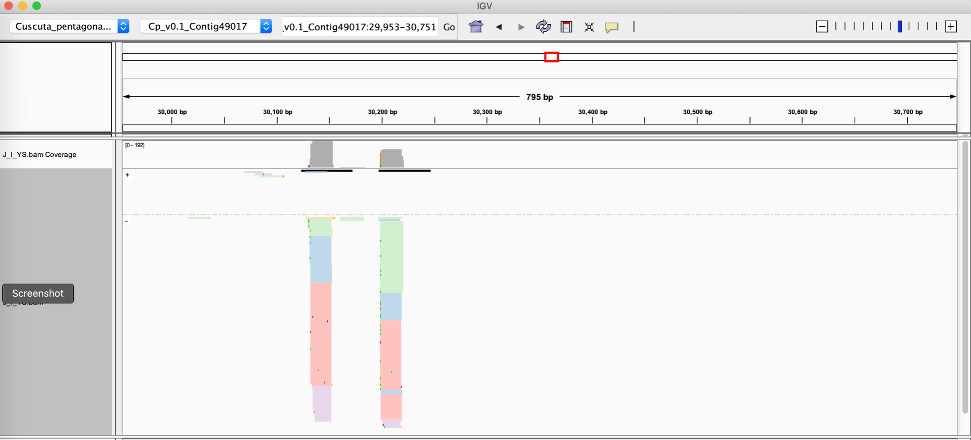
Let’s assume you have a sRNA-seq analysis of two conditions, and thus have two different alignment files that you want to visually compare. The alignment files are in the standard BAM format, and they are both indexed. One very easy way to visualize these alignments is to use the Integrative Genome Viewer, which is a free download and very easy to set up on a laptop or desktop computer. Loading up two BAM files of sRNA-seq data with default settings on IGV will give you a view like this :

An IGV snapshot

When given a BAM file, IGV will automatically calculate a coverage track, which is a barchart showing the depth of reads at each nucleotide position. IGV’s defaults also represent the strands of the individual alignments with different colors (blue and red). There are some problematic aspects to this display:

  • Small RNA size cannot be rendered automatically by IGV. For plants, the size of the small RNAs is critical information: 21 nucleotide RNAs are strongly associated with post-transcriptional silencing, while 24 nucleotide RNAs are associated with transcriptional silencing. 22 nucleotide RNAs are associated with amplification of silencing by triggering secondary siRNA formation. And most sRNA-seq datasets contain large numbers of RNAs shorter than 20, or longer than 24 nucleotides; these off-sized RNAs are generally not involved in gene regulatory processes. To sum up, showing small RNA sizes is critical for interpretation of sRNA-sew alignments, but IGV cannot do this.
  • The strand of the alignment is also critical. Plant siRNAs are processed out of longer double-stranded RNA precursors, and so they will align to both strands of the genome in a local cluster. In contrast, microRNAs are processed from stem-loop single-stranded RNA precursors, so they will align to a single genomic strand. Degraded bits of other RNAs, which are common in sRNA-seq datasets, will align to only one strand of the genome. The default IGV view does show strand of individual alignments (in color). However, this can be misleading when there is a large stack of alignments at the same position: IGV may be only able to render a small fraction of the reads (the rest are “stacked” out of the window), and the strands of the visible ones may not be a representative subset of the whole population. Ideally, we want the strandedness to be apparent in the coverage, not the individual alignments.
  • Lack of space. It’s very difficult to show more than two BAM files on the same screen. But many experimental setups have many more than two alignments.
  • Scaling.  IGV will auto-scale each loaded BAM file independently. This makes it very hard to visually identify differences in small RNA accumulation when comparing BAM files.

Below, I’ll walk through several approaches that, collectively, address all of these issues and enable more informative visualization of plant sRNA-seq alignments.

Modifying BAM files by read length

The first step we take is to add a custom tag to each alignment in the BAM files. The tag “YS” was chosen by me to categorize each aligned small RNA. There are five categories defined:

  • “<21nts” :: RNAs less than 21 nucleotides long. These are generally not known to be Argonaute-loaded and are thus more likely to be other types of RNAs, including degraded bits of random RNAs.
  • “21nts” :: RNAs that are exactly 21 nucleotides long. In plants this size is associated primarily with post-transcriptional silencing without the triggering of secondary siRNAs.
  • “22nts” :: RNAs that are exactly 22 nucleotides long. In plants this size is associated primarily with post-transcriptional silencing WITH triggering of secondary siRNAs.
  • “23-24nts” :: RNAs that are exactly 23 or 24 nucleotides long. In plants these sizes are associated primarily with transcriptional silencing and RNA-directed DNA methylation that occurs in the nucleus.
  • “>24nts” :: RNAs longer than 24 nucleotides. These are generally not known to be Argonaute-loaded and are thus more likely to be other types of RNAs, including degraded bits of random RNAs.

The script ‘add_YS.pl’ (available from the sRNA_Viewer GitHub repo) will add YS tags to a BAM file, like so: (more details are on the Github page)

add_YS.pl -b alignments.bam

Once modified with these custom tags, IGV visualizations can be improved. For instance, using the right-click menu for a BAM track in IGV, one can:

  • ‘Group alignments by’ –> ‘tag’ and enter YS
  • ‘Color alignments by’ –> ‘tag’ and enter YS

As shown below, this allows the aligned reads to be colored and grouped based on their size categories.

a genome browser snapshot

Grouping and coloring sRNA-seq reads by YS tag (size classes)

Switching the ‘Group alignments by’ to ‘Read strand’, both the read size categories and the strand can be visualized.

a genome browser snapshot

Coloring reads by YS tag (size category) and grouping them by Read strand.

Better views with sRNA_Viewer.R

Adding YS tags helps the IGV visualizations, but does not solve all of the problems. In particular, the problems of no room for more than ~2 tracks and different scalings between tracks remain. To solve this, I wrote a few more bits of code in the sRNA_Viewer repository. There is a two-step process that uses one or more YS-modified BAM files as input:

  1. Compute the per-nucleotide depth of coverage by strand, read-size category, and BAM file (script sRNA_coverage.pl) and output as a tab-separated text file.
  2. Use those data to make a coverage plot (script sRNA_Viewer.R).

The process can be run as a single pipeline (details given on the GitHub repo):

sRNA_coverage.pl -b bamfileList.txt -c Chr1:10993-11087 | sRNA_Viewer.R -p output.pdf

This will produce a PDF file where each BAM file has its own figure, the y-axis (RNA coverage in units of reads-per million) is scaled the same for all plots, and for which the strand is denoted by + and – numbers (for + strand and – strand reads, respectively). An example, with 12 different BAM files showing a microRNA locus that is differentially expressed in different libraries, is shown below:

small RNA coverage plot

Output from sRNA_Viewer.R , showing sRNA depth of coverage by size category and strand for 12 different BAM files.

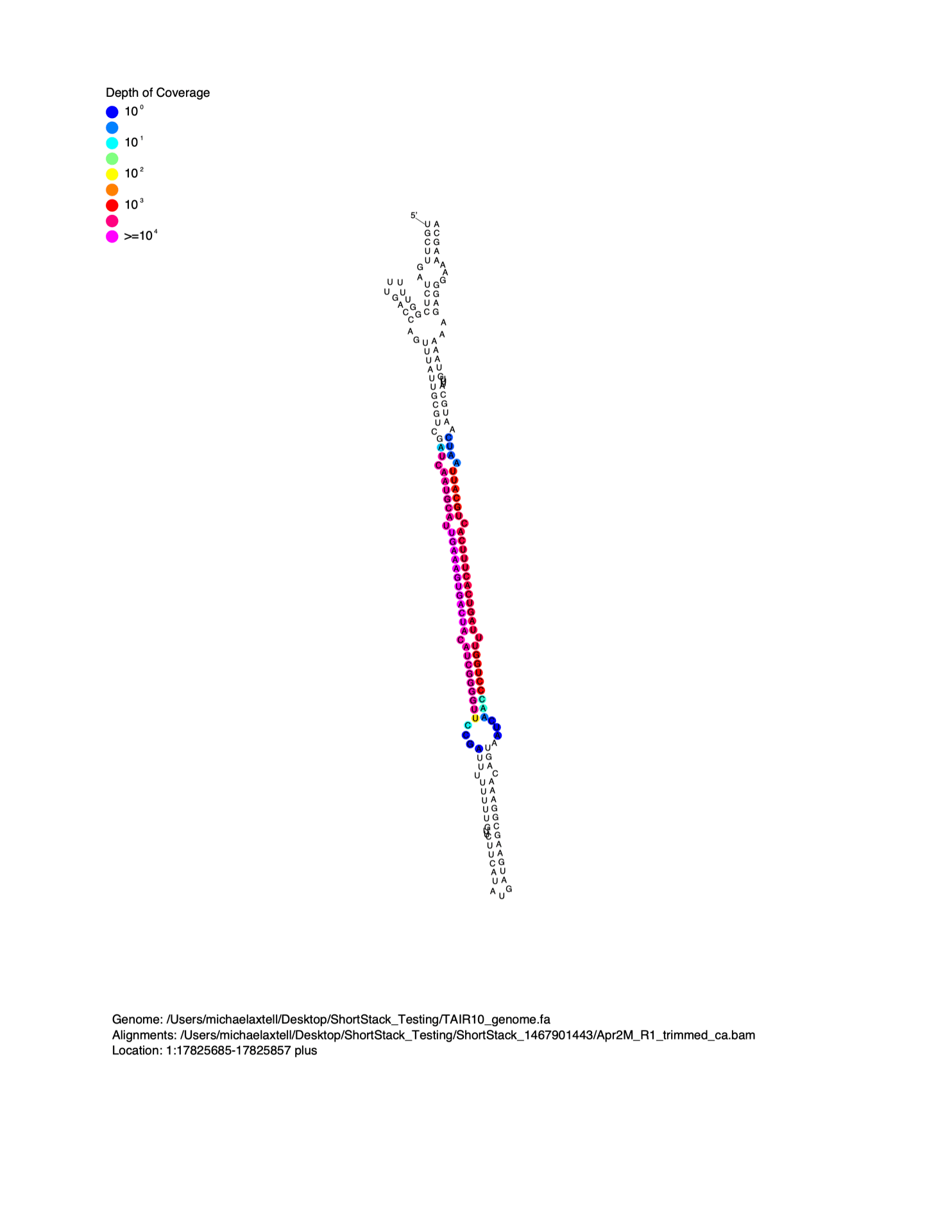
Viewing sRNA alignment depth in the context of predicted precursor secondary structure

MicroRNAs are distinguished from short interfering RNAs (siRNAs) by the unique secondary structures of microRNA precursors. MicroRNAs are processed out of the helical regions of “stem-loop” RNA secondary structures in precursors. When viewed on a linear alignment (as in the examples above), this results in a characteristic “two-peak” pattern. The two peaks represent the microRNA, and the partner strand created during biogenesis (the so-called microRNA*). It is often helpful to visualize small RNA alignment depth as a function of predicted precursor RNA secondary structure. To do this, I wrote the script strucVis . This script takes in a BAM file, the corresponding genome (in FASTA format), coordinates and genomic strand of interest, and an optional name, and makes two outputs:

  1. A post-script formatted image showing the predicted RNA secondary structure of the locus, with sRNA-seq alignment depths color-coded on each nucleotide.
  2. A plain-text representation of the predicted RNA secondary structure with aligned sRNA reads shown underneath.

Details on the usage of strucVis can be found at the GitHub repository.

Example image from strucVis

strucVis image output


Improving ShortStack performance on highly fragmented genomes

Highly fragmented reference genomes (with thousands or more short contigs or scaffolds) have been a persistent challenge for our small RNA-seq analysis program ShortStack. During a run, ShortStack needs to retrieve genomic sub-sequences for analysis of predicted RNA secondary structure. This is required to identify MIRNA hairpins. Early on I made the decision to use the samtools faidx function as the engine to retrieve genome sub-sequences. This was just pragmatic and lazy .. samtools was already required for other portions of ShortStack’s analysis, and there wasn’t a need to reinvent the wheel. However, when we started to do runs against highly fragmented genome assemblies, we found analysis was very slow. The slowness was traced to the samtools faidx function, which is very sensitive to the number of contigs/references.

The first attempt to fix this issue was in version 3.0, when I introduced the use ‘genome-stitching’.  When the reference genome had more than 50 sequences, and some were < 1Mb in size, the references were ‘stitched’ together into larger assemblies of at least 5Mb each. This worked very well to speed up the process of MIRNA searching, but had some disadvantages:

  1. The end results (bam file, results, etc), were in the coordinate system of the ‘stitched’ genome, not the original. This was quite inconvenient for users.
  2. The reads had to be aligned to the ‘stitched’ genome, which necessitated building a new bowtie index — this added total time to the run.
  3. I recently noticed a bug as well .. despite my efforts to prevent it, sometimes de novo small RNA clusters were found that spanned the junctions between ‘stitched’ genome segments.

In release 3.8, I’ve removed the drawbacks of the old stitching approach, while keeping the speed-up. The solution was simple and I’m kicking myself for not thinking about it earlier. Fragmented genomes are still stitched during the run (now into larger chunks, > 50Mb), but the stitched version is used only for sequence lookups. To get a sequence, the ‘real’ coordinates are converted to the ‘stitched’ coordinates, and the stitched genome used for the samtools faidx query. This keeps the speed up in retrieving sequences for folding, but the results are still reported in the original genome’s coordinate system. This approach eliminates all 3 of the problems listed above.

To demonstrate the speed-up, I compared the performance of 3.8 to 3.7.2 run with nostitch with the following conditions, using a highly fragmented reference genome I’m working on with a collaborator at the moment:

  • Reference genome: 382,375 scaffolds, totaling 3.75Gb of sequence. bowtie indices pre-built.
  • Alignments: 202,147,307 reads (pre aligned in single bam file).
  • mincov = 0.5rpm

Performance:

  • 3.7.2 (under nostitch) : 3 hrs, 14 minutes
  • 3.8 (improved stitch, still reporting in original coordinates): 1 hr. 13 minutes

So, the performance gain is clear, nearly three times as fast. Because so many new genome assemblies are highly fragmented drafts, this performance enhancement may matter to many users.


NO BAR CHARTS! (Weissgerber et al. 2015)

I came across this article in PLoS Biology (Weissgerber et al. 2015 doi: 10.1371/journal.pbio.1002128) and it very clearly laid out the issues of using barcharts to display continuous data, especially with low sample sizes. Bottom line: barcharts are misleading summaries of the data, and it’s better to show the data themselves with univariate scatter plots or boxplots. Figure 1 from their paper dramatically shows how barcharts can mask very different distributions of the data:

Figure 1:  Weissgerber et al. (2015).

Figure 1: Weissgerber et al. (2015).

Figure 3 from this paper is also very striking. Here we can easily see the fallacy of using standard error of the mean (SEM), or standard deviation (SD) for non-normally distributed, low sample size data:

Figure 3: Weissgerber et al. (2015)

Figure 3: Weissgerber et al. (2015)

Some people in my lab probably remember me complaining about barcharts for qRT-PCR experiments where n=3 or n=6 on one of our recent papers. I prevailed, and we had scatter plots instead of barcharts. Maybe now my motivations are clearer? 🙂

Figure 7D from our recent paper (Coruh et al. 2015 Plant Cell doi: 10.1105/tpc.15.00228) .. note avoidance of barchart!

Figure 7D from our recent paper (Coruh et al. 2015 Plant Cell doi: 10.1105/tpc.15.00228) .. note avoidance of barchart!

ShortStack now on iPlant

A big thanks to Nate Johnson for coordinating the loading of ShortStack 3.3 onto iPlant’s Discovery Environment. There is now a ‘public app’ for ShortStack on the discovery environment. Just search ‘ShortStack’ in the apps.

This will allow users to leverage iPlant’s compute resources instead of their local machines to run ShortStack. It also uses a gui interface instead of the command line to run the software.

Anyone who uses this, please let me know! (mja18@psu.edu) .. would love to track how much use the community is getting out of the iPlant app.

CRISPR/Cas9 ‘toolbox’ of vectors for plants

Since today’s seminar speaker here is Dr. Daniel Voytas from Minnesota, I went looking for some of his recent papers. I came across this recent one, from him and his collaborators, reporting a series of vectors optimized for plant transgenesis with various types of CRISPR activities, including multi-plexed targeting and transcriptional activation. At a glance the experiments look convincing, and the vector series is available at Addgene. Folks in my lab who are interested in multi-plexed CRISPR/Cas9 targeting might want to look at this study.

A CRISPR/Cas9 Toolbox for Multiplexed Plant Genome Editing and Transcriptional Regulation. (2015; Plant Physiology. doi: 10.1104/pp.15.00636)

Untitled

Plant miRNA evolution update

So here’s another figure I’ve prepared for the Plant Cell review article I am writing. This is an update on the patterns of miRNA conservation across land plants according solely to the information present in miRBase release 21.

For this analysis, I first placed each land plant miRNA family in miRBase 21 into one of eight broad plant groups (Eudicots-Rosids, Eudicots-Asterids, Basal Eudicots, Monocots, Basal Angiosperms, Gymnosperms, Lycophytes, and Bryophytes). I then defined a conserved miRNA family as one which had at least one high-confidence annotation, and which was annotated in two or more of these broad groups. By this definition, there are just 36 conserved families out of the more than 2,000 that are currently annotated.

grid_fig

This figure also highlights a major issue in the large-scale analysis of land plant miRNA conservation .. highly unequal sampling density within the different groups. Rosids and monocots have received the most attention, with large numbers of species represented, and high numbers of overall annotations (barcharts at the top). In contrast, basal eudicots, basal angiosperms, lycophytes, and bryophytes are much less well-sampled, with each group represented at present by just one species in miRBase 21. Inferring secondary losses in some of these lineages (basal eudicots, basal angiosperms, lycophytes) is NOT believable.

This chart also illustrates how important the high-quality miRNA annotation set for bryophytes is (the sole species represented is Physcomitrella patens). Based on the presence of high-confidence annotations in both Physcomitrella and one or more angiosperm group, we can confidently say that nine families (miR156, miR160, miR166, miR171, miR319, miR390, miR477, miR529, and miR535) were most likely present in the last common ancestor of all land plants. Another three families (miR167, miR395, and miR408) might also belong in the ultra-conserved set, but they are less certain because their Physcomitrella annotations are not high-confidence. Another two families (miR396 and miR482) clearly predate divergence of all seed plants. Other patterns are less certain because of the frequent presence of annotations that are not (yet) known to be high confidence. I think this again highlights the need for a systematic review of miRNA annotations, based on re-analysis of all available small RNA-seq data with a single, high-confidence MIRNA identification methodology. We are working toward this goal in my lab.

Plant microRNAs in miRBase 21

So I’ve been asked to contribute a review article to The Plant Cell on the general subject of microRNA / small RNA evolution in plants.  I set out to make an up to date figure on microRNA annotations across plants based solely on the annotations in miRBase 21. The results were surprising to me.

72 different land plant species are represented in miRBase 21, with a total of 2,247 different miRNA FAMILIES annotated. Note, that is families, not loci. Seemingly a huge diversity of different miRNA sequences.

But, the issue is that many of these annotations are likely to be false positives .. either other types of regulatory small RNAs, or even worse, just degraded garbage. The curators of miRBase, since release 20, have set out to try and make a ‘high-confidence’ list of microRNA loci, based on their internal parsing of public small RNA-seq data. (See their paper in NAR). In miRBase 21, from plants, there are just 176 high-confidence miRNA families (a high-confidence family is a family for which at least one locus has a high-confidence designation).  Furthermore, only 17 of the 72 plant species have ANY high-confidence annotations at all! The scatterplot below illustrates this, as we can see that most species have few annotated families and no high-confidence ones.

miRBase_scatterplot

Scatterplot of numbers of high-confidence miRNA families from 72 plant species as a function of the total number of annotated families. Data are coded according to broad taxonomic groups. A few species of interest are labeled. Data were processed from miRBase 21.

Of course, there are some caveats here. The biggest is that the ‘high-confidence’ designation is based on whether or not the miRBase folks have analyzed the available high-throughput small RNA-seq data for a given species. In some cases, they may not have (though I haven’t dug into that specifically). The second caveat is that all species are NOT equally treated here. Some species (for instance, Oryza sativa, Arabidopsis thaliana) have high-quality reference genomes and have had lots of experimental attention over the years. Many others have neither of these traits, and so their annotations are necessarily more piecemeal. Overall I think this points out the need clearly for a more uniform approach to retrospective analysis of miRBase annotations.

I was also pleased to see that Physcomitrella patens has a very high percentage of high-confidence miRNA families .. since my lab annotated the vast majority of those families!

— Mike Axtell

High temps trigger 24mer siRNAs in Arabidopsis?

I came across this article, published about a year ago, in Plant Physiology and Biochemistry and was intrigued:

Insight into small RNA abundance and expression in high- and low-temperature stress response using deep sequencing in Arabidopsis

doi: 10.1016/j.plaphy.2014.09.007

The experiment was small RNA-seq on heat-stressed (HT .. 36C for one day), normal temperature (NT) and low-temperature (LT .. 4C for one day ) Arabidopsis plants. The basic observation that I found intriguing was that the high-temp stress library had quite a few 24mers, while the cold and normal temp. libraries had a lot fewer. (See Figure 1 from the paper below):

Baev_Fig1

Does this imply that heat stress activates the 24nt siRNA pathway?

The major issue with the experiment however is a lack of replication and independent verification: Just one library per treatment so there are no biological replicates to assess the reproducibility, so the result I think is provisional at best.

However, there are some earlier reports that also show effects of heat stress on bulk small RNA functions. Ito et al. (2011) showed that the Arabidopsis ONSEN retrotransposon was transcribed and reverse-transcribed in response to heat stress, but that actual transpositions were prevented by the het-siRNA pathway. Zhong et al. (2013) showed that heat stress de-activated the trans-acting siRNA pathway (which mostly makes 21 and 22mer siRNAs that can also behave like heterochromatic siRNAs). I think that understanding the role of heat-induced small RNA profile changes will be quite interesting.

Rcount: dealing with multi-mapping reads in RNAseq data

Rcount: simple and flexible RNA-Seq read counting

Marc W. Schmid* and Ueli Grossniklaus

Institute of Plant Biology and Zu€rich-Basel Plant Science Center, University of Zurich, 8008 Zu€rich, Switzerland

Bioinformatics. doi:10.1093/bioinformatics/btu680, PMID: 25322836

Nate showed me this paper today which is of some interest to us given my obsession with finding a better way to deal with the issue of multi-mapping reads in small RNA-seq data (e.g., with the butter program). This paper describes a tool called Rcount, which is a counter for ‘normal’ mRNA-seq data. As described in the paper, Rcount takes in a BAM file, and deals with multireads. According to figure 1 (copied below), the way they do this is to use the density of local uniquely mapped reads and make a probability assessment… the more uniquely mapped reads in an area, the more likely it is that the multi-read also came from that location. They then place it, noting their calculated probability in the SAM line with a custom tag. Rcount then performs another task (dealing with counting reads that overlap more than one gene annotation) and counts up reads in annotated genes for the user.

Rcount is clearly geared toward counting reads in annotated genes with reference to mRNA-seq data. For that reason, I doubt the program itself will be that useful for small RNA-seq data, where we are not generally interested in counting reads in pre-defined intervals (like gene annotations). But it is striking that Rcount is using pretty much exactly the method that my butter program uses for assigning reads … using the density of the unique mappers to create a probability set used to guide decisions on multi-mappers. I think Nate is going to try and use Rcount for small RNA-seq data.

I don’t think this precludes continued development of butter or it’s successor, because Rcount is pretty clearly geared toward mRNA-seq data. But it is worth testing, if possible, against butter and other methods for small RNA-seq to try and determine for our own lab purposes an optimal method for aligning multi-mapped small RNA-seq reads that is both precise and reproducible.

– Mike Axtell

plantDARIO – a web-based tool for small RNA-seq analysis in select plant genomes

Patra et al. (2014). plantDARIO: web based quantitative and qualitative analysis of small RNA-seq data in plants. Frontiers in Plant science.

doi: 10.3389/fpls.2014.00708
PMID: 25566282

This manuscript describes a web-based service for the annotation of small RNA-producing genes in Arabidopsis thaliana, Beta vulgaris, and Solanum lycopersicum (the authors also state that they plan to extend the number of plant species to “…include most of the available plant genomes.”. Users provide aligned small RNA data in BAM or bed format, and the authors provide a script for condensing reads aligned to the same position. Thus the authors reduce the burden of large data transfers. The web server parses the aligned small RNA data with respect to several pre-loaded annotation tracks, including known miRNAs (from miRBase), known tasi-RNAs, tRNAs, and other ncRNAs from Rfam. Global stats are spit out for the library. Clusters of reads that don’t overlap any annotated regions are flagged, and some miRNA finding and snoRNA finding programs are run. Results can be integrated onto other publically available genome browsers for the species of interest, located on other servers.

I found this manuscript interesting for a couple of reasons. First, I had often wondered about how to make my own small RNA-seq program, ShortStack, available as a web-service. I have not done this, primarily because the input for ShortStack is raw small RNA-seq data, or BAM files of aligned small RNA-seq data, along with the reference genome. This would be tedious to upload for users because of the file sizes. The large file sizes could also place a big demand of the server, as could the intense number of CPU cycles that might be run. It looks like the authors of plantDARIO have gone around this issue by outsourcing the alignments to the user, and enforcing a read-condensation scheme.

The second thing I found interesting about this work was a brief mention of the alignment methods. In particular, the authors state “Unlike many other mapping tools, segemehl has full support for multiple-mapping reads which is very important for small RNA-seq”. I am quite interested in improving the treatment of how multi-mapped small RNA-seq reads are placed and used (see butter). I have not heard of the program “segemehl” before. The relevant paper is Otto et al., 2014, which I will need to put on my reading list.

The third thing I was interested in was the method for annotating small RNA clusters that didn’t overlap a known gene. The authors are using a tool called “blockbuster”, which was described in another earlier paper from this group, Langenberger et al. 2009. Will have to check this out too.

My final thoughts on this paper have to do with comparing a web-based service like plantDARIO to a stand-alone program like ShortStack. The authors of this paper make a plug for a web-based service and ding stand-alone programs by stating “The other sncRNA prediction tools need to be downloaded, installed and run locally, requiring more than basic computer skills.” Well yes, this is true. But there are significant advantages of a stand-alone vs. their approach to web-based analysis. With a standalone, you can use any genome assembly or assembly version you want. But with their approach, you are limited to whatever they have pre-configured. Moving to new species, or even updating with a newer genome assembly version, is not possible except by requesting the authors to update their site. There is a lot more flexibility to be gained with a standalone.

In any event, an interesting read. I’m looking forward to trying out the tool, and to reading some more of the background methods, especially alignments and de-novo cluster finding.

PS. One error: My ShortStack paper is erroneously cited as “Allen et al. (2013)” instead of “Axtell (2013)”. The author lists of my paper and a 2004 paper from the Carrington Lab, with Ed Allen as lead author, appear to have been swapped in the ref. cited section.

–Mike Axtell