The last few updates to Mathematica have added some useful cartographic tools for map making. Some of my earlier posts included some simple maps. For any serious cartography, you need to be able to plot the boundaries of various “administrative” units that make up a region – these can be states, provinces, counties, cities, etc. Mathematica, like python can do just about anything that you really set your mind to, so if you have geographic information in existing files, you can parse it and display it with the GeoGraphics command. In this note I show how to acquire information on basic administrative units, in particular, their coordinates, so they can be displayed on the maps you use to show your own data (earthquake locations, seismic stations, etc).

When I make a map, I usually have a set of bounds that define the region of interest (influenced strong by the Generic Mapping Tools) by specifying the west, east, south, and north edges. Let’s start with an example defining a geographic rectangle and requesting a list of the countries that overlap our region. In  the example I was exploring seismic stations available in northeast China so the box covers that region. Instead of plotting seismometer locations, I’ll plot country boarders and large city locations. We’ll need the country list, country polygons, and a list of large cities and their populations.

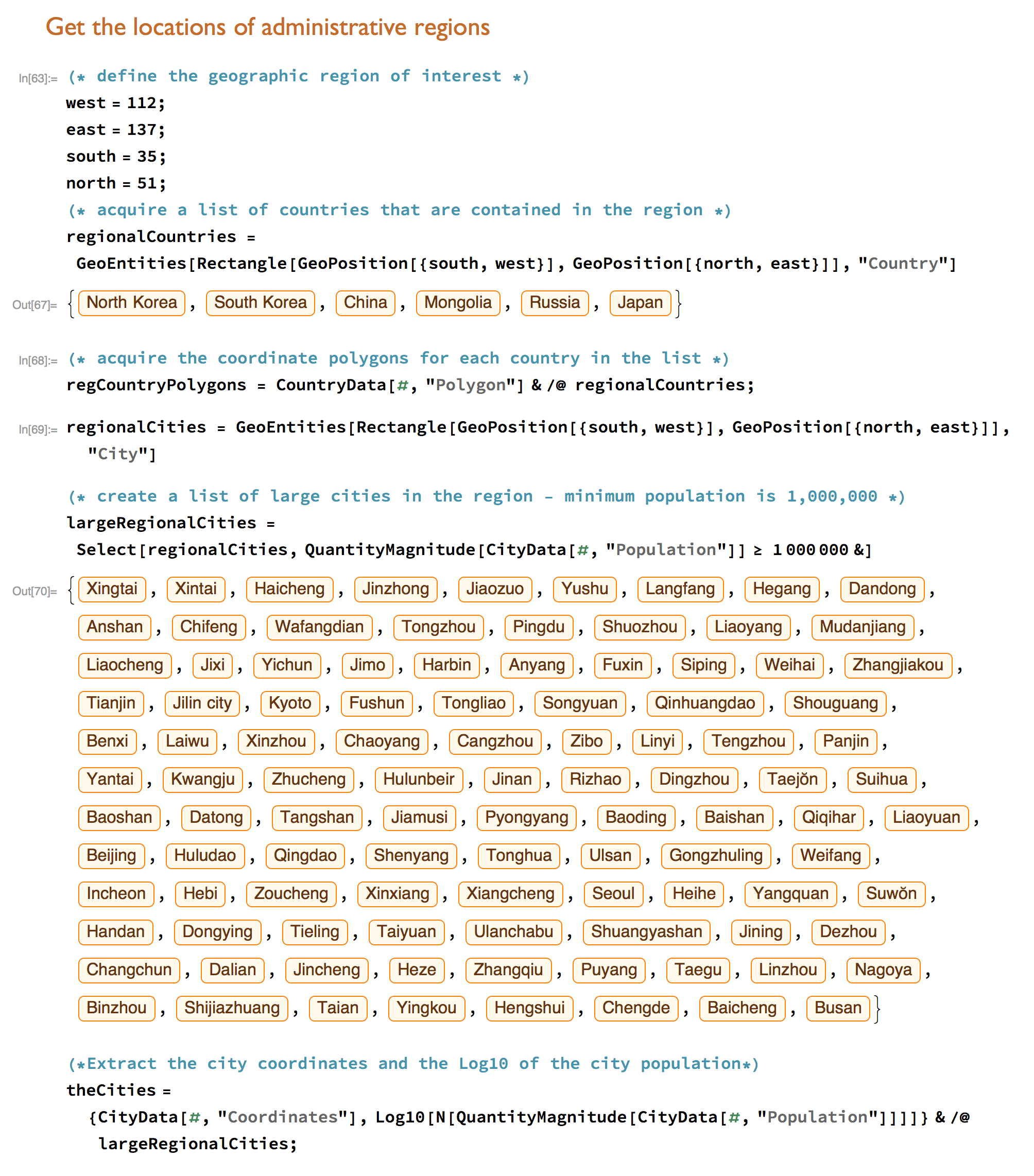
(* define the geographic region of interest *)
west = 112;
east = 137;
south = 35;
north = 51;

(* acquire a list of countries that are contained in the region *)
regionalCountries = 
 GeoEntities[Rectangle[GeoPosition[{south, west}], GeoPosition[{north, east}]],
        "Country"]

(* acquire the coordinate polygons for each country in the list *)
regCountryPolygons = CountryData[#, "Polygon"] & /@ regionalCountries;

regionalCities = GeoEntities[Rectangle[GeoPosition[{south, west}], GeoPosition[{north, east}]], 
 "City"]
(* create a list of large cities in the region - 
          minimum population is 1,000,000 *)
largeRegionalCities = Select[regionalCities,
     QuantityMagnitude[CityData[#, "Population"]] >= 1000000 &];

You can see what properties are available from CityData using

In[1]:= CityData["Properties"]

Out[1]= {"AlternateNames", "Coordinates", "Country", "Elevation", "FullName", 
"Latitude", "LocationLink", "Longitude", "Name", "Population", "Region", 
"RegionName", "StandardName", "TimeZone"}

Here’s what the output in the notebook looks like. The “data” requests return Mathematica “Entities“, which are information objects that can be queried for additional information, as we did asking the countries for cities and asking the cities for populations and coordinates. Entities are represented by the orange rounded rectangles in the notebook.

We can plot the information using the GeoGraphics command. I use a Mercator projection, which is relatively simple. At least at this time, Mathematica cannot label latitudes along the frame of a map, so I create my own labels and the pass them to the GeoGraphics command.  Since I am doing my own latitude labels, I might as well do my own longitude labels and use a more professional size tick mark (Mathematica has awful default tick mark sizes).

(*Extract the city coordinates and the Log10 of the city \
population*)theCities = {CityData[#, "Coordinates"], 
 Sqrt[N[QuantityMagnitude[CityData[#, "Population"]]/10^6]]} & /@ 
 largeRegionalCities
(* create latitude tick locations and labels *)
latTicks = Join[Table[{N[GeoGridPosition[GeoPosition[{ilat, west}],
   "Mercator"]][[1]][[2]], ilat, {0.0, 0.02}}, {ilat, south, north, 5}],
   Table[{N[GeoGridPosition[GeoPosition[{ilat, west}],
   "Mercator"]][[1]][[2]], "", {0.0, 0.01}}, {ilat, south,north, 1}]
   ];

lonTicks = Join[Table[{N[GeoGridPosition[GeoPosition[{south, ilon}], 
    "Mercator"]][[1]][[1]], ilon, {0.0, 0.02}}, {ilon, 10, east,5}],
    Table[{N[GeoGridPosition[GeoPosition[{south, ilon}], 
    "Mercator"]][[1]][[1]], "", {0.0, 0.01}}, {ilon, west, east,1}]
   ];

(* draw the map *)
GeoGraphics[{ {FaceForm[None], EdgeForm[Thick], regCountryPolygons},
  {GeoStyling[Opacity[0.65], FaceForm[Red], EdgeForm[{Black, Thin}]], 
      GeoDisk[{#[[1]][[1]], #[[1]][[2]]}, 4*Quantity[#[[2]], "km"]] & /@ theCities} },
  GeoRange -> {{south, north}, {west, east}},
  BaseStyle -> {21, FontFamily -> "Helvetica"},
  GeoProjection -> "Mercator",
  Frame -> True, FrameTicks -> {{latTicks, None}, {lonTicks, None}},
  GeoZoomLevel -> 6,
  GeoBackground -> {GeoStyling["ReliefMap", 
      GeoStylingImageFunction -> (Lighter[#1, 0.1] &)]},
  ImageSize -> 600] // Print

and here is the map

Large cities (population >= 1M) in northeast China.

You can get a list of China’s Province boundaries using

chinaStates = Entity["Country", "China"]["AdministrativeDivisions"];
chinaStatePolys = AdministrativeDivisionData[#, "Polygon"] & /@ chinaStates;

I like the fact that I can get geographic-related information from Mathematica. But Mathematica’s geographic data are not perfect, the state on country borders do not overly one another perfectly. Something for Wolfram to work on…

Noted added after initial post

The code below scales the city symbols so that the area of the circle is proportional to the population in millions.

(*Extract the city coordinates and the Log10 of the city population*)
theCities = {CityData[#, "Coordinates"], 
    Sqrt[N[QuantityMagnitude[CityData[#, "Population"]]/10^6]]} & /@ largeRegionalCities

The symbol-size variations are not too large, but they are enough to indicate that the population variations are substantial.

Large cities (population ≥ 1M) in northeast China. Symbol area is proportional to population.