Purpose of Calculation

Geometric optimization of a unit cell is useful for finding the minimum energy configuration of a molecule or solid without needing to manually change atom positions. Through numeric minimization algorithms, the proper lattice parameters and atom positions can be obtained. For molecules, this can also find the minimum energy bond angles and bond lengths. However, the different contexts between solids and molecules can present very different challenges. These calculations will compare the convergence and speed of the geometry optimization calculations of water and hydrogen cyanide (HCN), using two different basis sets: Castep’s [1] plane wave basis set and DMol3’s calculated-on-the-fly localized basis set [2].

Figure 1: Optimized geometry of a water molecule

Figure 2: Optimized geometry of a hydrogen cyanide molecule in the H-C-N isomer

Figure 3: Optimized geometry of a hydrogen cyanide molecule in the H-N-C isomer

Calculation Methodology

The bond angle and bond lengths of water and hydrogen cyanide are calculated using two different basis sets.

All calculations are performed with the Perdew-Burke-Ernzerhof (PBE) [3] exchange-correlation functional, a Generalized Gradient Approximation (GGA) functional. The Koelling-Harmon relativistic treatment was used for atomic solutions [4] in the Castep calculations for the plane wave basis set. The on-the-fly basis set is calculated by generating a radial function calculated by solving the density equations on the fly at three hundred points on a logarithmic radial mesh for each atom. This radial function is then multiplied by appropriate spherical harmonics for each atom.

Convergence Calculations

Calculations to check the convergence of the minimum energy output with respect to the energy cutoff, the k-point mesh and the unit cell size were performed for the Castep calculations. It is necessary to check the convergence with respect to the unit cell size because the plane wave basis fills the entire cell. Due to the computational assumption of repeating cells, each unit cell must be large enough so that each molecule does not interact with those in adjacent cells. Convergence tests must be used to idea what is a sufficiently large cell. These tests are shown in figures 4-9 for both water and hydrogen cyanide.

Fig. 4 Convergence of Castep with respect to Cutoff Energy for water

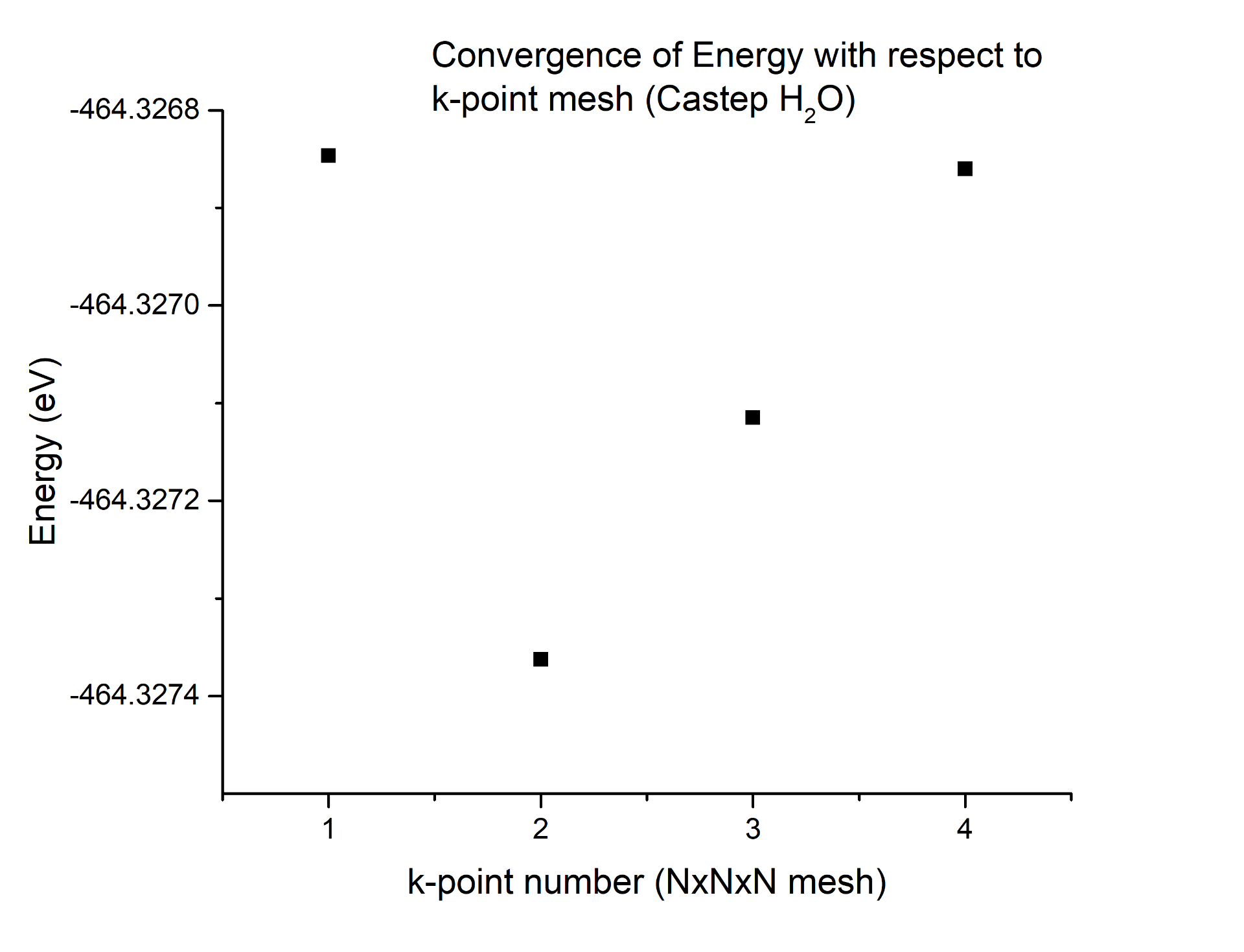
Fig. 5 Convergence of Castep with respect to k-point number for water

Fig. 6 Convergence of Castep with respect to unit cell size for water

Fig. 7 Convergence of Castep with respect to Cutoff Energy for hydrogen cyanide

Fig. 8 Convergence of Castep with respect to k-point number for hydrogen cyanide

Fig. 9 Convergence of Castep with respect to unit cell size for hydrogen cyanide

For DMol3, we do not need to converge the unit cell size. The generated basis sets are highly localized, and we instead test the convergence of the maximum radius of the radial functions, referred to as the cutoff radius. The cutoff radius must be large enough that each atom “sees” the other atoms during all of the geometry optimization, but can still be smaller enough that the basis does not extend as far as the unit cell extends in the Castep calculations. As a result, we check the convergence of energy calculations with respect to cutoff radius and k-point mesh. These convergence tests are shown in figures 10-13 for both water and hydrogen cyanide.

Fig. 10 Convergence of DMol3 with respect to k-point number for water

Fig. 11 Convergence of DMol3 with respect to cutoff radius for water

Fig. 12 Convergence of DMol3 with respect to k-point number for hydrogen cyanide

Fig. 13 Convergence of DMol3 with respect to cutoff radius for hydrogen cyanide

All parameters were converged to within 0.01 eV

Calculation Results

The key metric for comparing the two sets of results is the computational time for both the geometry optimization and the convergence tests. Given an arbitrarily long time, either basis set can give an equally accurate and precise calculation of the bond angles and bond lengths. The important comparison is how quickly the computations can be performed using each basis set to within reasonable agreement with each other.

Both basis sets agree that there is one minimum for the water molecule: a planar bent structure, with bond angle of approximately 104 degrees and a bond length of approximately 0.97 angstroms. Both basis sets also report two isomers of hydrogen cyanide, the H-C-N configuration, and the C-N-H configuration, both with a linear orientation and bond angle of approximately 180 degrees. Disagreement on the exact bond angles and lengths is minor, but does occur. Exact results are included in table one. By better converging the minimum energy, a geometry optimization with a stricter cutoff could be run in order to lessen such disagreement. This, however, is not the purpose of this example case.

The total computation time for both convergence studies and the geometry optimizations for Castep is 8486 seconds (141.43 minutes). For DMol3, the total time is 102 seconds, providing a similar degree of accuracy. This result is expected, due to the more localized basis set being favorable for describing the more local behavior of a molecule confined to a small portion of a cell. The size of the disparity between the two methods is very noteworthy, however, and shows how helpful it can be to choose the correct basis set for a give task.

References

[1]  S. J. Clark, M. D. Segall, C. J. Pickard, P. J. Hasnip, M. J. Probert, K. Refson, M. C. Payne, “First principles methods using CASTEP”, Zeitschrift fuer Kristallographie 220(5-6) pp. 567-570 (2005)

[2]  Delley, J., Fast Calculation of Electrostatics in Crystals and Large Molecules; Phys. Chem. 100, 6107 (1996)

[3]  John P. Perdew, Kieron Burke, and Matthias Ernzerhof, “Generalized Gradient Approximation Made Simple”, Phys. Rev. Lett. 77, 3865 – Published 28 October 1996; Erratum Phys. Rev. Lett. 78, 1396 (1997)

[4]  D D Koelling and B N Harmon 1977 J. Phys. C: Solid State Phys. 10 3107

In this work we use density functional theory to find the preferred geometry of molecular pairs of hydrogen cyanide (HCN) and water (H₂0). We performed these calculations for all electrons within the framework of DMol³⁽¹·²⁾ using a basis set of atomic orbitals and the PBE⁽³⁾ functional for the exchange-correlation energy. The specific basis set used was DNP 3.5 (double numerical with polarization).

Methods

As a precursor to our main result, we performed geometry optimization for isolated H₂O and then isolated HCN and compared our results to values in the literature. This served a dual purpose, not only providing us with a suitable initial geometry for each of the molecules in our main calculation, but also giving us an idea the systematic errors implicit in our method. Our calculations corroborate and are corroborated by the values reported in the literature, as may be seen in Table 1.

Table 1: Geometry of HCN and H2O

Table 1: Geometry of isolated HCN and H₂O

Because the geometry optimization algorithms proceed by using calculated forces to update initial atomic positions, it is critical that we choose judiciously the set of initial geometries we will optimize. Individual initial geometries must be chosen so that appreciable forces exist, and the set of initial geometries must be diverse enough to capture all local minima. Here we discuss our choice of initial geometries.

As free parameters our we may choose the three-variable locations (e.g. three Cartesian coordinates) and two-variable orientations (e.g. polar and azimuthal angles) of each molecule. This is immediately reduced by the fact that only the relative displacement and orientations of the molecules matter, and we exploit this freedom by choosing to place the carbon of HCN at the origin initially and align it with the z-axis. Furthermore, because HCN is linear, it is identical upon rotations about this axis and hence we can also take H₂O to be in the xz plane. Symmetry in reflection across the yz plane means we can further narrow the space to be considered to the portion of the xz plane with x>0. We are left with four parameters for H20, two for each of its location and its orientation.

With the bond lengths and angles fixed, we chose five initial positions for the water molecule, each with two orientations. At a distance of 2-3Å from the carbon of HCN, H₂O was placed at approximately 30°, 60°, 90°, 120° and 150° from the z axis. For each location one optimization began with the H₂O dipole either parallel or antiparallel to the x axis, with the plane defined by the three atoms of H₂O at a 45° angle to the xz plane. Two examples are shown below in Figure 1.

Figure 1 – Two example initial geometries; with C of HCN as the origin, the upper H₂O is at 30° off the z-axis (measured as the angle O-C-N) with a dipole parallel to the x-axis and the lower H₂O is at 120° with a dipole antiparallel to the x-axis

Our minimization criterion was to have the energy and displacement between successive steps vary by less than, respectively, 10⁻⁵Ha and 0.002Ha/Å. Those interested in reproducing our results should note that, with our maximum step size of 0.3Å, in a few cases (namely, those in which H₂O was initially repulsed by dipole forces) this took slightly over 50 iterations to converge.

Results

All equilibria we found fell into one of three categories. The lowest in energy had a hydrogen bond between the H of HCN and O of H₂O with an energy of -169.7358Ha; the dipole of H₂O formed an angle of approximately 30° with the axis of HCN. This is shown in Figure 2. The angle between the dipoles can be qualitatively explained by thinking of the tetrahedral geometry of oxygen’s two bonds and two lone pairs under sp³ hybridization. If H₂O were a regular tetrahedron and one lone pair were aligned with the HCN axis, some geometry leads to 35° as the expected angle, so the tetrahedral shape of a molecule with sp³-hybridized orbitals explains our results well.

In the next lowest, a hydrogen bond formed between an H of H₂O and the N of HCN, with the relevant O-H bond aligned with the linear HCN. The energy of this arrangement was -169.7337Ha. This difference is about 0.05eV, or about 660K on the Boltzmann energy scale. (There is of course an “activation energy” necessary to switch configurations which exceeds this gap, but this is not the subject of this project.)

Figure 2 – The two miminal-energy geometries of H₂O and HCN

All but one of the convergent optimizations described above ended with the lowest-energy state; only when H₂O was placed at 30° off the z-axis with its two Hs (its positive poles) facing the N of HCN (its negative pole). When the opposite orientation was assumed (i.e. O closest to N) the repulsive force so outweighed any force in the z-direction that H₂O simply drifted away from HCN. An additional calculation the dipole of H₂O orthogonal to that of HCN, with H₂O centered 25° off the z-axis, also converged to this secondary local minimum. Thus the H₂O-NCH geometry (here the atoms connected by hyphens share a hydrogen bond) is the stable energy miminum for a large majority of initial geometries, with a moderately strong but not insurmountable difference between the two minima.

Conclusion

We have determined that the most energetically favorable arrangement of a single molecule each of H₂O and HCN is that in which O in H₂O forms a hydrogen bond with H in HCN. We also showed that a second local energy minimum exists in which one of the two H in H₂O forms a hydrogen bond with N in HCN. The existence of multiple local minima suggests that a many-molecule system could have very interesting geometries – for example, one might imagine that it could more energetically favorable for some molecules to take the slightly higher-energy arrangement if it would allow more energy-lowering hydrogen bonds to occur elsewhere. The possibities could be further expanded by considering HCN’s higher-energy tautomer hydrogen isocyanide, structurally written NCH. The single-H₂O, single-HCN nature of our work elucidates the “building blocks” of such many-particle interactions and builds a good foundation for future work on increasingly complex systems.

References

[1] B. Delley, “An all‐electron numerical method for solving the local density functional for polyatomic molecules”.J. Chem. Phys. 92, 508 (1990).

[2] B. Delley, “From molecules to solids with the DMol³ approach”. J. Chem. Phys. 113, 7756 (2000).

[3] J. P. Perdew, K. Burke and M. Ernzerhof, “Generalized gradient approximation made simple”. Phys. Rev. Lett. 77, 3865 (1996).

[4] L.E. Sutton, ed., “Tables of Interatomic Distances and Configuration in Molecules and Ions”. London: The Chemical Society (1958). (via www.wiredchemist.com/chemistry/data/carbon-compounds)

[5] A. G. Császár, G. Czakó, T. Furtenbacher, J. Tennyson, V. Szalay, S. V. Shirin, N. F. Zobov and O. L. Polyansky, “On equilibrium structures of the water molecule”. J. Chem. Phys., 122, 214305 (2005). (via http://www1.lsbu.ac.uk/water/ref9.html#r836)

1. Problem Description

In this project, we aim to predict the optimal structures of H₂O and HCN using DFT. To calculate the energy of an isolated molecule with periodic supercells, the molecule is placed in a large enough cubic supercell to minimize the influence from period images. To perform the geometric optimization, we need to take all the internal degrees of freedom like bond lengths and bond angles into consideration with appropriate stopping criterions for energy and force. We start from various initial structures with all degrees of freedom included to see if they will finally converge to the same structure to ensure that we reach the optimal structures.

The Vienna Ab initio Simulation Package (VASP) is used to perform periodic DFT calculations,^1-3 employing the projected augmented-wave (PAW) pseudopotentials and the generalized gradient approximation with exchange-correlation functional by Perdew, Burke, and Ernzerhof (PBE).^4-6 The conjugated gradient algorithm is chosen to perform the geometric optimization in VASP.

2. H₂O Structure

Before we can perform the geometric optimization of H₂O, convergence tests are required firstly with respect to the size of the unit cell as well as the energy cutoff. The test for number of k-points is not required here because all the calculations for such geometric optimization of one molecule in a large box use a 1x1x1 k-point sampling. For both H₂O and HCN, all three atoms lie in one plane. In order to do the convergence test, we initially put the O atom at the (0, 0, 0) and two H atoms at (1/L, 0, 0) and (-1/L, 0, 0) according to the experimental results (H-O bond length usually around 1 Å) as shown in Figure 1 (L is the side length of the unit cell).

Figure 1. H₂O in a large box (H₂O is located at the vertex of the cubic unit cell)

Energy cutoffs ranging from 400.00 to 600.00 eV are used and the side length of the cubic unit cell is chosen from 20.0 to 30.0 Å with an increment of 1 Å. The results of the convergence tests are summarized below in Table 1-2 and Figure 2-3.

Table 1. Convergence tests on energy cutoff for H₂O

Table 2. Convergence tests on unit cell size for H₂O

Figure 2. Energy vs energy cutoff for H₂O                  Figure 3. Energy vs unit cell size for for H₂O

Based on these results, we chose the energy cutoff of 500.00 eV (tolerance of 0.005 eV) and the side length of 25.0 Å for further calculation of the water molecule.

Now, we firstly vary the bond length between H and O atoms while still keeping them linearly arranged on the y-axis. The O atom remains (0, 0, 0) and the two H atoms are located at (a/L, 0, 0) and (-a/L, 0, 0). Here, L=25.0 Å and a is chosen from 0.5 to 1.3 Å with the interval of 0.1 Å. The results are summarized below in Table 3.

Table 3. Results for H₂O with different initial bond lengths

From these results, we can see that the energies for the cases with initial bond lengths of 0.5 and 0.6 Å are significantly higher as the distances between atoms in the optimal geometry, which are trapped in a local minimum, are much larger than typical bond lengths as shown in Figure 4. The distances between the O atom and the H atom are 9.790 and 4.809 Å for these two cases, respectively. As two H atoms are initially too close to the O atom, this situation physically represents the enormously compressed bonds, which brings a strong repulsive force pushing the atoms away from each other. The numerical optimization method then takes an initial step that separates the two atoms by a very large distance and they can never go back since the force is much weaker now due to the very large distance. All other cases give us the same optimized structure as shown in Figure 5. The H-O bond length is 0.943 Å and the bond angle q_HOH is 180.00°.

Figure 4. Separated H₂O with initially short distances   Figure 5. Optimized structure for H₂O

In order to ensure that the structure above is the optimal structure, we modify the initial structure through changing the bond angle that does not make components of the forces vanished by symmetry. So, with the O atom remaining at (0, 0, 0), the two H atoms are at (a/L, b/L, 0) and (-a/L, b/L, 0). L here is the side length of 25.0 Å, and according to the results above, the a is fixed at 0.9 Å while b is chosen from 0.1, 0.2, and 0.3 Å to have three different initial bond angles. After optimization, we find that these three tests finally converge at the same free energy of -14.217 eV with the same optimized structure of H₂O as shown in Figure 6. The H-O bond length is 0.972 Å and the bond angle q_HOH is 104.50°. The energy is lower than the previous cases with bond angle of 180.00° and since three different bond angles finally converges to the same structure, this is the optimal structure for H₂O. The experimental H-O bond length and bond angle is 0.958 Å and 104.48°, respectively. We see that the DFT-predicted bond length and bond angle are very similar to the experimental results with differences less than 2%.

Figure 6. Optimal structure for H₂O

3. HCN Structure

Similarly, the convergence tests are required before we optimize the structure HCN. Due to the similar size of these two molecules, the convergence test on unit cell sizes is no longer required and the side length of 25.0 Å above is used. We similarly put the C atom at the (0, 0, 0), the N atom and the H atom are at (1/L, 0, 0) and (-1/L, 0, 0) as shown in Figure 7 (L is the side length of the unit cell and is fixed at 25.0 Å here).

Figure 7. HCN in a large box (HCN is located at the vertex of the cubic unit cell)

Energy cutoffs ranging from 400.00 to 600.00 eV are tested for HCN. The results are summarized below in Table 4 and Figure 8. Based on these results, we chose the energy cutoff of 500.00 eV using the same tolerance for further calculations of HCN.

Table 4. Convergence tests on energy cutoff for HCN

Figure 8. Energy vs energy cutoff for HCN

Again as we did for the H₂O molecule, we vary the N-C and H-C bond lengths while keeping all of them on the y-axis. The C atom remains (0, 0, 0) and the N and H atoms are located at (a/L, 0, 0) and (-a/L, 0, 0). Here, L=25.0 Å and a is chosen from 0.7 to 1.5 Å with the interval of 0.1 Å. The results are summarized below in Table 5.

Table 5. Results for H₂O with different initial bond lengths

From these results, we can see that the energies for the cases with initial bond lengths of 0.7, 0.9, and 1.0 Å are significantly higher due to the large distances between atoms as shown in Figure 9. These atoms are pushed apart from each other with the similar reason for those H₂O with very short bond lengths (only one H-C bond, the N atom is far away). For the case of 0.8 Å, it even cannot converge. The optimized structures for the rest cases are totally the same as shown in Figure 10. The N-C and H-C bond lengths are 1.161 and 1.075 Å, respectively. The bond angle q_HCN is 180.00°.

Figure 9. Separated HCN with initially short distances    Figure 10. Optimized structure for HCN

Similarly, we then modify the initial structure by changing the bond angle to make sure that the force components are not canceled out by symmetry. So, with the C atom remaining at (0, 0, 0), the N and H are at (a/L, b/L, 0) and (-a/L, b/L, 0). L here is the side length of 25.0 Å, and according to the results above, the a is fixed at 1.2 Å while b is chosen from 0.1, 0.2, and 0.3 Å to have three different initial bond angles. After optimization, we find that all these three tests finally give the same free energy of -19.690 eV and the same optimized structure of HCN as shown in Figure 11. The N-C and H-C bond lengths are 1.161 and 1.075 Å, respectively. The bond angle q_HCN is 179.95°. The energy is almost the same compared to the previous cases with bond angle of 180.00° and since three different bond angles finally converges to the same structure, this is the optimal structure for HCN. The experimental N-C and H-C bond lengths are 1.156 and 1.064 Å, and the bond angle 180.00°. We see that the DFT-predicted bond length and bond angle are very similar to the experimental results with differences less than 2%.

Figure 11. Optimal structure for HCN

4. Conclusion

To conclude, in this project, we find the optimal structures of H₂O and HCN. For H₂O, the DFT-predicted H-O bond length is 0.972 Å and the bond angle q_HOH is 104.50° (the experimental values are 0.958 Å and 104.48). For HCN, the DFT-predicted N-C and H-C bond lengths are 1.161 and 1.075 Å while the bond angle q_HCN is 179.95° (the experimental values are 1.156 and 1.064 Å, and 180.00°). We see that the DFT can accurately predict the bond lengths and bond angles for these selected molecules with differences less than 2% compared to experimental results.

Reference

1. Kresse, G. and J. Hafner, Ab initio molecular dynamics for liquid metals. Physical Review B, 1993. 47(1): p. 558.
2. Kresse, G. and J. Hafner, Ab initio molecular-dynamics simulation of the liquid-metal–amorphous-semiconductor transition in germanium. Physical Review B, 1994. 49(20): p. 14251.
3. Kresse, G. and J. Furthmüller, Efficient iterative schemes for ab initio total-energy calculations using a plane-wave basis set. Physical review B, 1996. 54(16): p. 11169.
4. Kresse, G. and D. Joubert, From ultrasoft pseudopotentials to the projector augmented-wave method. Physical Review B, 1999. 59(3): p. 1758.
5. Blöchl, P.E., Projector augmented-wave method. Physical review B, 1994. 50(24): p. 17953.
6. Perdew, J.P., K. Burke, and M. Ernzerhof, Generalized gradient approximation made simple. Physical review letters, 1996. 77(18): p. 3865.