
After beginning operations earlier this year, HPF continues to patiently watch for the subtle Doppler shifting of stellar spectra that hints at the back-and-forth tug of orbiting exoplanets. As described in previous blog posts, HPF records spectra on a detector array (similarly to how a digital camera records an image), and the shifts we seek amount to microscopic motions of the spectra back and forth by just a few nanometers!
To be able to detect this shifting, we have engineered HPF to be very stable – the optics and detector are built from special materials and mounted carefully so that they don’t cause any shifts of the spectra that could be misinterpreted as Doppler shifts. We’ve carefully thought about all the potential causes of “false” Doppler shifts, from slight thermal changes moving the diffraction grating to systematically weird ways that the light can be launched from the fiber into the spectrograph.
However, this precision engineering doesn’t eliminate the “false” Doppler shifts, which are often referred to as “drifts” of the spectrograph. Even with a perfectly still, unmoving stellar spectrum shining into the telescope, we would still observe the spectrum moving in position by a few nanometers on the detector. These drifts may be attributable to any number of physical causes, from mechanical relaxation of optical components to slight differences in the weight distribution of the optical bench when we fill up HPF with liquid nitrogen coolant every day.
No matter the cause, these drifts must be corrected if we hope to detect the true ~1 meter per second signals from habitable zone planets orbiting M dwarfs. We go about correcting the measurements by measuring the spectra of two sources at once: one being the star of interest, and the other being a calibration source that is known to stay as still as possible. Any measured drifts of the calibration spectrum should be entirely due to “false” Doppler shifts. We can then subtract these from the measured shifts of the stellar spectrum, which contains both the “true” Doppler shift of the stellar spectrum as well as the drift. This isolates the “true” Doppler shift of the star (or more precisely, the relative motion between the star and the Earth).
What types of spectra can we use for this calibration?
An ideal calibration spectrum should have spectral lines throughout the region we are measuring, and those lines should be as stable as possible. The lines should also be roughly uniform in brightness, because we don’t want the detector to be blinded by one spectral line that is much brighter than the others.
Historically, the main option available for such calibration has been atomic emission lamps. These lamps are filled with certain well-characterized element mixtures (such as Thorium + Argon), and when an electrical current is passed through this mixture, it emits light at wavelengths corresponding to the energy levels of the atoms. Unfortunately, the wavelengths of these lines can change over time as the lamps age (the composition or pressure within the lamp can change slightly), and the lines are neither regularly positioned nor of equivalent brightness (see bottom panel of figure below).
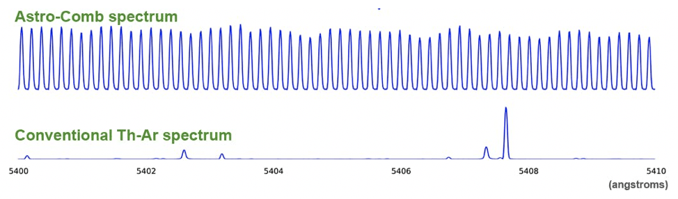
An example comparison of calibration spectra for astronomical spectrographs.
Far better is the new generation of calibration sources, called laser frequency combs (LFCs), or “astro-combs.” These sources produce spectra with emission lines that are evenly spaced, roughly of uniform brightness, and stable in their positions. These properties result from the physical mechanisms that generate the comb, and there are several different pathways for generating the comb.
The HPF Astro-Comb
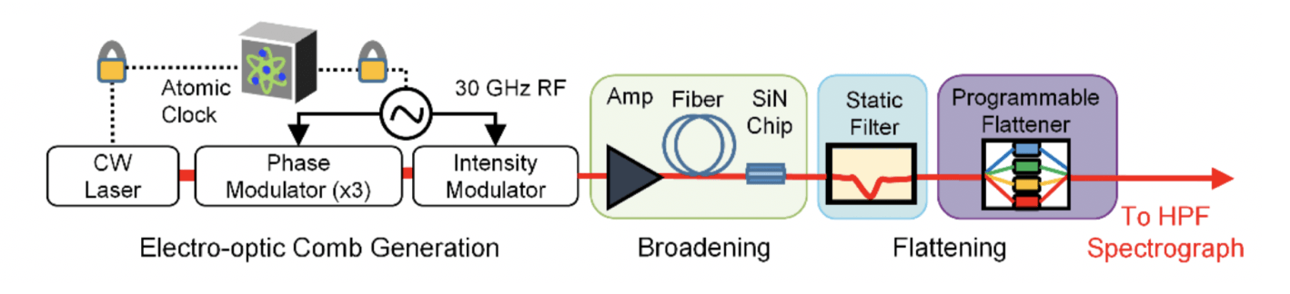
The schematic of the HPF Astro-Comb.
HPF is outfitted with a laser frequency comb developed by our team members at NIST. This one-of-a-kind comb was developed in parallel with the spectrograph itself, and is really an instrument unto itself! As shown in today’s other post, the combination of the HPF spectrograph and astro-comb unlocks the full potential of the instrument.
The HPF comb uses the so-called “electro-optic” technique. It is based on a single continuous-wave laser (at one wavelength/frequency, in this case approximately 1064 nanometers or 282 terahertz). A set of modulators blink the laser on and off, and also shift the phase of the laser wave back and forth. The effect of this is that the calibration spectrum goes from being one wavelength to being a comb of many wavelengths (i.e. the modulation generates “sidebands”). The separation between these lines is equivalent to the rate of the modulation, and the main requirement on this is that it has to be sufficient that we can resolve the comb lines with HPF. This means that the HPF comb modulators have to operate at 30 GHz (they swing back and forth 30 billion times each second), an impressive feat!
After the laser modulation, the calibration spectrum is a comb, but it only spans about 10 nanometers in wavelength, while a full HPF spectrum covers almost 500 nanometers. Clearly, another step is needed in order to broaden the HPF comb spectrum. This is where a neat device called a nonlinear waveguide comes in to play. By shining the “narrow” comb into the nonlinear waveguide (which is made of silicon nitride), we are able to stack and shuffle the comb lines together (a process called four-wave mixing) to generate new comb lines and a much broader spectrum that spans the full HPF range. This process requires a lot of light, however, so first the comb has to be amplified to 2 watts – enough power to really burn your eyes! (So we have carefully built a safe system – the laser turns off automatically if you open its opaque box)
The full spectrum then spans the HPF range, and it is important to note that the whole system is connected to an atomic clock. This means that the various components are able to operate with knowledge of precisely how the best clocks in the world are ticking – so it knows and can control precisely the wavelengths (or frequencies) of all the comb lines. So not only do we have comb lines over the full HPF spectral range, but they are also completely stable!
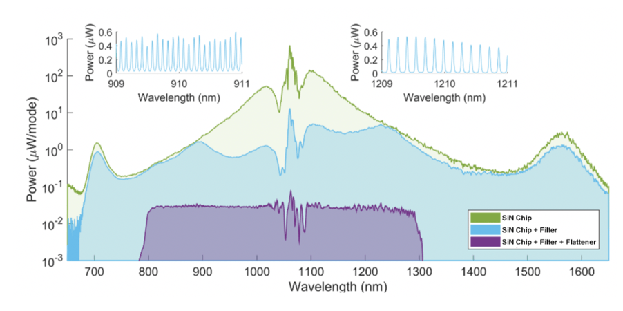
The spectral profile of the HPF comb.
However, this comb spectrum is very bright near its central wavelength around 1064 nanometers, and much fainter towards 820 and 1300 nanometers. So the final step is that we need to make sure that the comb lines are all roughly the same brightness. We use a combination of a static filter and an active liquid-crystal-display-type filter (actually a mini-spectrograph!) to make the brightness of the comb lines as equal as possible.
As you can tell from this description, this system has many interlocking parts, and it is one of the most advanced astro-combs yet demonstrated.
Installation and performance of the HPF comb
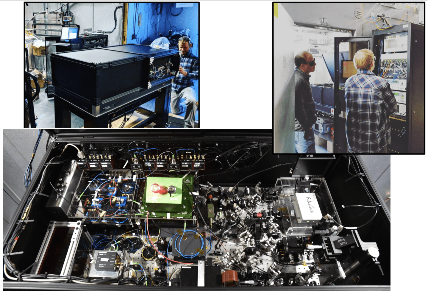
Photos from the installation of the HPF astro comb.
The HPF comb was installed in February of 2018, and underwent some engineering upgrades in April and May of 2018. A few photos of the deployment are shown above. The comb has been running smoothly since May, and the impressive measurements it has enabled are detailed in an accompanying blog post (see for example the simultaneous stellar and astro-comb spectra from HPF below). Our recent paper also describes the performance of this system in much more detail.
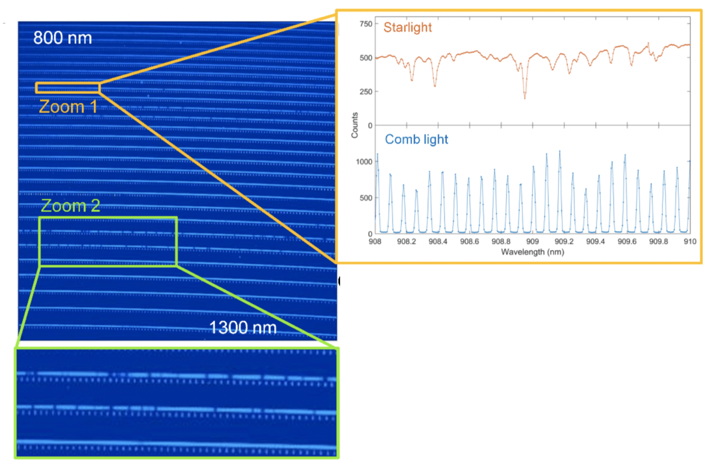
Side-by-side spectra of a star and the HPF astro-comb.
 RSS - Posts