
LAB 1:
ALTOONA CRIME RATES
R MODULE 1:
ACCESSING DATA
In this tutorial, we import data on Altoona crime rates into RStudio, and then inspect the data using summary statistics. RStudio is an integrated development environment (IDE) for the R programming language – essentially, RStudio is a more user-friendly interface for programming in R.
We will first (1) set our working directory, then (2) create a new R script in RStudio, and finally (3) use the R code presented further below in this Module.
(1) Setting a working directory in RStudio
Open RStudio. You will notice the following tabs:
- Console, where code is executed and output often provided.
- Environment, where created variables, data frames, etc. are listed.
- Plots, where graphs are usually plotted.
- Files, where your current working directory is shown (the Files tab doesn’t actually say “working directory” anywhere, but this is what the Files tab is showing you by default).
You can see other tabs, but do not worry about them now.

Working directory, as the name implies, is the location in which R is working by default. If you don’t tell R otherwise, this is from where it will take files, and this is to where it will save files.
To set the working directory to the folder with our
datasets, do the following:
- On RStudio’s main ribbon, click Session > Set Working Directory > Choose Directory

- A new window pops up. Navigate to the folder containing our datasets, and click OK:

The Files tab (on the right) is now showing our new working directory contains our 2 datasets.
The Console tab (on the left) shows how we could have set the working directory using R code (this code would have achieved the exact same result we just did in RStudio manually).

Great, your working directory is now set!
Generally, you always want to set your working directory. This is for 2 reasons:
- Calling a file that is in your working directory makes the code shorter, and
- Reproducing code with a working directory is easier for other programmers.
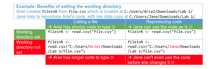
In conclusion, setting up the working directory saves time, and is a good programming practice.
(2) Creating a new R script in RStudio
There is one main tab still missing – the one for writing our R script. To add that, do the
following:
- On RStudio’s main ribbon, click File > New File > R Script.

The new Untitled tab appears – this is where you will be writing your R script:

Great, your R script is ready for coding! The benefit of coding in an R script is that you can always save it for later use, without the need to rewrite the code.
(3) Coding in R
Now that we have set up RStudio, time to code in R!
Copy and paste the below script into your new Untitled R script tab in R Studio.
- Every line of code starting with the pound key / hashtag (#) is interpreted as a comment in R. It does not affect the code, or the output. It serves as instructions. Read the comments in each block before you execute the code.
- There is an example of output after each block of code. Make sure your own output in R matches the output presented here.
- You execute a line in R script by being in that line, and pressing CTRL+Enter.
R Script (copy below code, paste, and execute in RStudio; do not copy the output results)
# # # # # NSF Project “Big Data Education” (Penn State University)
# # # # # More info: http://sites.psu.edu/bigdata/
# # # # # Lab 1: Altoona Crime Rates – Module 1: Accessing Data
# # # # STEP 0: SET WORKING DIRECTORY
# Set working directory to a folder with the following file:
# ‘Lab 1 Data Altoona Crime Rates.csv’
# # # # STEP 1: READ IN THE DATA
# Below command says: “define variable AltoonaCrimeRates
# which reads as a csv file ‘Lab 1 Data Altoona Crime Rates.csv’,
# uses comma (,) as field separator, and has a header row”
# (a first row containing names of all columns).
# The <- syntax means assigning something to something else in R.
AltoonaCrimeRates <- read.csv(“Lab 1 Data Altoona Crime Rates.csv”,sep=”,”, header=TRUE)
|
OUTPUT (a new data frame
<![if !vml]>
|
 <![endif]>
# See the data set you just read into R
AltoonaCrimeRates
|
OUTPUT (shows first 25 rows for all 39 variables):
1 Jan-13 01B-Manslaughter by Negligence M 0 1 0 0 2 Jan-13 030-Robbery M 2 0 0 0 3 Jan-13 030-Robbery F 1 0 0 0 4 Jan-13 040-Aggravated Assault M 10 0 1 0 5 Jan-13 040-Aggravated Assault F 1 0 0 0 6 Jan-13 050-Burglary M 4 2 2 2 7 Jan-13 050-Burglary F 1 0 0 0 8 Jan-13 060-Larceny-Theft M 22 2 2 2 9 Jan-13 060-Larceny-Theft F 17 0 0 1 10 Jan-13 070-Motor Vehicle Theft M 2 0 1 0 11 Jan-13 070-Motor Vehicle Theft F 1 0 0 0 12 Jan-13 080-Other Assaults – Not Aggravated M 49 7 1 1 13 Jan-13 080-Other Assaults – Not Aggravated F 14 0 0 1 14 Jan-13 090-Arson M 2 0 0 0 15 Jan-13 110-Fraud M 1 1 0 0 16 Jan-13 110-Fraud F 4 0 0 0 17 Jan-13 130-Stolen Prop., Rec., Posses., Buying M 5 1 2 1 18 Jan-13 140-Vandalism M 3 4 1 2 19 Jan-13 140-Vandalism F 1 0 0 0 20 Jan-13 150-Weapons, Carrying, Posses, Etc. M 4 1 1 0 21 Jan-13 150-Weapons, Carrying, Posses, Etc. F 1 0 0 0 22 Jan-13 170-Sex Offenses (Except 02 and 160) M 1 0 0 0 23 Jan-13 18B-Drug Sale/Mfg – Marijuana M 2 0 1 0 24 Jan-13 18C-Drug Sale/Mfg – Synthetic M 2 0 )0 25 Jan-13 18D-Drug Sale/Mfg – Other M 4 0 0 0
1 0 0 0 0 0 0 0 0 0 0 0 2 0 0 0 0 0 0 1 1 0 0 0 300000010000 4 5 6 7 8 9 10 11 12 13 14 15 16 0 0 0 0 0 17 18 19 20 21 22 23 24 25
1 2 3 4 5 6 7 8 9 10 11 12 13 14 15 16 17 18 19 20 21 22 23 24 25 Adult.Race.Asian.Pacific Adult.Ethnic.Hispanic 1 2 3 4 5 6 7 8 9 10 11 12 13 14 15 16 17 18 19 20 21 22 23 24 25
1 2 3 4 5 6 7 8 9 10 11 12 13 14 15 16 17 18 19 20 21 22 23 24 25 Juvenile.Race.Native.American Juvenile.Race.Asian.Pacific 1 2 3 4 5 6 7 8 9 10 11 12 13 14 15 16 17 18 19 20 21 22 23 24 25 Juvenile.Ethnic.Non.Hispanic 1 2 3 4 5 6 7 8 9 10 11 12 13 14 15 16 17 18 19 20 21 22 23 24 25 [ reached
|
# See the data set you
just read into R, in a more organized table
View(AltoonaCrimeRates)
|
OUTPUT (a new tab is
<![if !vml]>
|
 <![endif]>
# Get summary statistics
of the data set
summary(AltoonaCrimeRates)
|
OUTPUT:
Nov-14 : 50 060-Larceny-Theft Aug-16 : 49 080-Other Assaults – Not Jul-14 : 49 210-Driving Under the Aug-15 : 48 220-Liquor Law May-14 : 47 260-All Other Offenses (Except Apr-16 : 46 230-Drunkenness (Other):2037 (Other) Juvenile.Total Min. : 1st Qu.: 0.0000 1st Qu.: 0.0000 1st Qu.: 0.000 1st Qu.: 0.0000 1st Qu.:0.0000 Median Mean : 3rd Qu.: 1.0000 3rd Qu.: 0.0000 3rd Qu.: 0.000 3rd Qu.: 0.0000 3rd Qu.:0.0000 Max. :26.0000 Max. :17.0000 Max. :22.000 Max. :12.0000 Max. :7.0000
Min. :0.0000 Min. :0.000 Min. :0.0000 Min. : 0.000 Min. : 0.000 Min. : 0.0000 1st Qu.:0.0000 1st Qu.:0.000 1st Qu.:0.0000 1st Qu.: 0.000 1st Qu.: 0.000 1st Qu.: 0.0000 Median :0.0000 Median :0.000 Median :0.0000 Median : Mean :0.2618 Mean :0.282 Mean :0.3022 Mean : 1.304 Mean : 1.137 Mean : 0.9058 3rd Qu.:0.0000 3rd Qu.:0.000 3rd Qu.:0.0000 3rd Qu.: 2.000 3rd Qu.: 1.000 3rd Qu.: 1.0000 Max. :6.0000 Max. :7.000 Max. :8.0000 Max. :30.000 Max. :21.000 Max. :21.0000
Min. : 1st Qu.: 0.000 1st Qu.:0.0000 1st Qu.: 0.000 1st Qu.:0.0000 1st Qu.:0.0000 1st Qu.:0.0000 Median Mean : 3rd Qu.: 1.000 3rd Qu.:1.0000 3rd Qu.: 0.000 3rd Qu.:0.0000 3rd Qu.:0.0000 3rd Qu.:0.0000 Max. :12.000 Max. :8.0000 Max. :10.000 Max. :6.0000 Max. :4.0000 Max. :4.0000
Adult.Race.White Min. : 1st Qu.: 1.000 1st Qu.: 0.0000 1st Qu.:0.000000 Median Mean : 3rd Qu.:10.000 3rd Qu.: 1.0000 3rd Qu.:0.000000 Max. :64.000 Max. :22.0000 Max. :1.000000
Adult.Ethnic.Hispanic Min. : 1st Qu.: 0.0000 1st Qu.: Median Mean : 3rd Qu.: 0.0000 3rd Max. :10.0000
Min. :0.0000 Min. :0.0000 Min. :0.0000 Min. : 0.0000 Min. :0.00000 1st Qu.:0.0000 1st Qu.:0.0000 1st Qu.:0.0000 1st Qu.: 0.0000 1st Qu.:0.00000 Median :0.0000 Median :0.0000 Median :0.0000 Median : Mean :0.1827 Mean :0.1935 Mean :0.2463 Mean : 0.7911 Mean :0.09716 3rd Qu.:0.0000 3rd Qu.:0.0000 3rd Qu.:0.0000 3rd Qu.: 1.0000 3rd Qu.:0.00000 Max. :9.0000 Max. :9.0000 Max. :8.0000 Max. :26.0000 Max. :5.00000
Juvenile.Race.Native.American Min. :0 1st Qu.:0 Median :0 Mean :0 3rd Qu.:0 Max. :0
Juvenile.Ethnic.Non.Hispanic Min. : 1st Qu.: 0.0000 Median Mean : 3rd Qu.: 1.0000 Max. :26.0000
|
# Get a count for all
values of variable “Offense.Code” from AltoonaCrimeRates
table(AltoonaCrimeRates$Offense.Code)
|
OUTPUT:
01A-Murder and Nonnegligent Manslaughter
060-Larceny-Theft
160-Prostitution and Commercialized Vice 170-Sex Offenses
18E-Drug
18G-Drug Possession –
200-Offenses
260-All Other
|
Challenges:
Use the outputs you just obtained to answer the following questions.
- By Offense Code: What are the most common, and least common crimes in Altoona (i.e. what Offense Codes appear in the dataset most and least times)?
- By Sex: Are crimes more often committed by men or women (i.e. what Sex appears in the dataset most times)?
- By Age: What group has committed the highest number of offenses for a single crime in a single month – adults, or juvenile offenders?
- By Age: What specific age group has committed the highest number of offenses for a single crime in a single month?
- By Race: What racial group has committed the highest number of offenses for a single crime in a single month?
- By Ethnicity: What ethnic group has committed the highest number of offenses for a single crime in a single month?
- What is the profile of the average person committing crimes in Altoona? Look at the max values for Offense Code, and Sex; average values for Adult vs. Juvenile, Age, Race, Ethnicity.
Important note for writing R code in
Word:
If you write your own R code in Word, you need to turn off Word’s autocorrecting of “straight quotes” (“”) into “smart quotes” (“”); otherwise, when you copy and paste the code into R, it will not work. This is because R only recognizes “straight quotes” (“”).
To disable “smart quotes”, in the main ribbon click File > Options:
<![if !vml]> <![endif]>
<![if !vml]> <![endif]>
In Options, click on Proofing > AutoCorrect Options:
<![if !vml]> <![endif]>
A new
window opens – in AutoFormat tab, un-check “Straight quotes” with “smart quotes”:
<![if !vml]> <![endif]>
In the same
window, in AutoFormat As
You Type tab, un-check “Straight
quotes” with “smart quotes” again:
Finally, click OK.
You are now all set to write your R script in Word!
Next Page: Previous Page: