Seismometers, Poles, & Zeros
Although not an everyday calculation, seismologists often benefit from a reminder of the instrument response curves (amplitude responses). Seismometers are generally described as the ratio of two polynomials in the Laplace Transform variable, s. The polynomials are described by their roots, which we call zeros (for the numerator polynomial) and poles (for the denominator polynomial). Generally when and instrument is calibrated, the information on the calibration is communicated by the poles, zeros, and an overall gain. To compare instruments with different gains, we also often choose a normalization frequency for display.
In the following I present some Mathematica scripts that I use to examine the poles, zeros, and instrument response amplitude spectrum. Slight modifications can introduce the phase information as well, but to keep things a little short, I leave that out of the description. We’ll look at four sets of instruments, Trillium, Steckheisen, and Guralp broadband seismometers, and then some short-period instruments that are part of the IRIS Consortium instrument pool.
Nanometrics Trillium Sensor Responses
I obtained the poles and zeros and zeros for the instrument responses from the PASSCAL web site and normalized the responses to a frequency of 1 Hz. Click here for the link.
Here is the code to set up three sets of poles and zeros as Mathematica lists – corresponding to the Trillium 120 PA, 240 (2nd Gen), and the Compact Trillium sensors.
(*
  Poles and zeros for the Trillium 120PA from
  http://www.passcal.nmt.edu/webfm_send/1970
*)
Zn120 = {0, 0, -90.0, -160.7, -3108};
Pn120 = {-0.03852 + 0.03658 I, -0.03852 - 0.03658 I, -178.,
         -135 + 160 I, -135 - 160 I, -671 + 1154 I, -671 - 1154 I};

(*
  Poles and zeros for the Trillium 240 (2nd Gen) from
  http://www.passcal.nmt.edu/webfm_send/1970
*)
Zn240 = {0, 0, -90., -164.2, -3203.};
Pn240 = {-0.01813 + 0.01803 I, -0.01813 - 0.01803 I, -124.9 + 0 I,
         -197.5 + 256.1 I, -197.5 - 256.1 I, -569 + 1150 I, -569 + -1150 I};
(*
  Poles and zeros for the Compact Trillium from
  http://www.passcal.nmt.edu/webfm_send/1970
*)
Znct = {0, 0, -434.1};
Pnct = {-0.036910 + 0.037120 I, -0.036910 + -0.037120 I, -371.2, -373.9 + 475.5 I,
   -373.9 - 475.5 I, -588. + 1508. I, -588.4 - 1508. I};
I can compute the three instrument responses using the following Mathematica functions. I could write one function and call it with the poles and zeros, but this is not that much extra work for an example. The second line in each function normalizes the response to unit amplitude at a frequency of one Hertz.
(* Instrument responses normalized at one Hz *)
Element[f, Reals];
s = I 2 \[Pi] f;
tr120resp[f_] = (Times @@ (s - Zn120)/Times @@ (s - Pn120)) /
                (Abs[Times @@ (s - Zn120)/ Times @@ (s - Pn120)] /. f -> 1.0);

tr240resp[f_] = (Times @@ (s - Zn240)/Times @@ (s - Pn240)) /
                (Abs[Times @@ (s - Zn240)/Times @@ (s - Pn240)] /. f -> 1.0);

ctresp[f_] = (Times @@ (s - Znct)/Times @@ (s - Pnct))/
             (Abs[Times @@ (s - Znct)/ Times @@ (s - Pnct)] /. f -> 1.0);
The variable \( s = i \omega \) is the Laplace Transform variable and has units of radians. I can display the instrument response amplitude spectrum using
p1 = LogLogPlot[{Abs[tr240resp[f]], Abs[tr120resp[f]], Abs[ctresp[f]]}, {f, 0.001, 1000 },
   Filling -> Axis, ImageSize -> 512,
   Axes -> False, Frame -> True,
   BaseStyle -> {14, FontFamily -> "Helvetica"},
   FrameLabel -> {"Frequency (Hz)", "Normalized Amplitude"},
   PlotLabel -> "Trillium Sensors" ,
   LabelStyle -> {14, FontFamily -> "Helvetica"},
   PlotLegends -> LineLegend[{"TR240", "TR120", "Compact"}]];
p1 // Print
Here is the plot.

Nanometrics Trillium seismometer response curves (amplitude).
A Pole-Zero Display
You can see the low-frequency corners for the the instruments near 240 and 1200 seconds, and some distortion on the TR instruments starting around 5Hz. We could also make a direct plot of the poles and zeros, which is interesting, but not at useful. I create two plots to show more detail around the origin (in the second panel). Here’s the graphics code.
(* Trillium 120 *)

mark = Graphics[{EdgeForm[GrayLevel[0.05]], FaceForm[LightBlue], Disk[{0, 0}, 0.05],
       PlotRangeClipping -> False}];

pltz = ListPlot[{Re[#], Im[#]} & /@ Pn120, AxesOrigin -> {0, 0},
   AspectRatio -> 1, Frame -> True,
   FrameLabel -> {{"Imaginary Part", None}, {"Real Part", "Trillium 120"}},
   BaseStyle -> {16, FontFamily -> "Helvetica"},
   PlotMarkers -> {mark, 0.04}];

mark = Graphics[{EdgeForm[GrayLevel[0.05]], FaceForm[Red], Disk[{0, 0}, 0.05],
       PlotRangeClipping -> False}];

pltn = ListPlot[{Re[#], Im[#]} & /@ Zn120,
    AxesOrigin -> {0, 0},
    AspectRatio -> 1,
    PlotMarkers -> {mark, 0.04}];

LabledSymbol[x_, y_, label_, color_] := {EdgeForm[GrayLevel[0.05]],
  FaceForm[color], Disk[Scaled[{x - 0.04, y} + 0.002], 120],
  Text[Style[label, {14, FontFamily -> "Helvetica"}],
   Scaled[{x, y}], {-1, 0}]}

p0 = Show[{pltz, pltn}, PlotRange -> {5000 {-1, 1}, 5000 {-1, 1}},
   Epilog -> {LabledSymbol[0.8, 0.9, "Poles", Red],
     LabledSymbol[0.8, 0.8, "Zeroes", LightBlue]}];

LabledSymbol[x_, y_, label_, color_] := {EdgeForm[GrayLevel[0.05]],
  FaceForm[color], Disk[Scaled[{x - 0.04, y} + 0.002], 7],
  Text[Style[label, {14, FontFamily -> "Helvetica"}],
   Scaled[{x, y}], {-1, 0}]}

p1 = Show[{pltz, pltn},
   PlotRange -> {300 {-1, 1}, 300 {-1, 1}},
   Epilog -> {LabledSymbol[0.8, 0.9, "Poles", Red],
   LabledSymbol[0.8, 0.8, "Zeroes", LightBlue]}];

GraphicsRow[{p0, p1}] // Print
Trillium seismometer poles and zeroes.
The Streckheisen STS2
We can compare the Trillium 120 with the Streckheisen STS2. Not much is different in terms of the code.
(*
  Poles and zeros for the STS2 3rd Generation from
http://www.passcal.nmt.edu/content/instrumentation/sensors/sensor-\
comparison-chart)
*)
PnSTS2 = {-13300, -10500 + 10100 I, -10500 - 10100 I, -520, -375, -97.3 + 401 I,
         -97.3 - 401 I, -15.6, -0.037 + 0.037 I, -0.037 - 0.037 I, -255};
ZnSTS2 = {0, 0, -463 + 431 I, -463 - 431 I, -177, -15.2};

(* Instrument responses normalized at one Hz *)
Element[f, Reals];
s = I 2 \[Pi] f;

sts2resp[f_] = (Times @@ (s - ZnSTS2)/
   Times @@ (s - PnSTS2)) /(Abs[Times @@ (s - ZnSTS2)/
      Times @@ (s - PnSTS2)] /. f -> 1.0);

p1 = LogLogPlot[{Abs[sts2resp[f]], Abs[tr120resp[f]]}, {f, 0.001, 1000 },
   Filling -> Axis, ImageSize -> 512,
   Axes -> False, Frame -> True,
   BaseStyle -> {14, FontFamily -> "Helvetica"},
   FrameLabel -> {"Frequency (Hz)", "Normalized Amplitude"},
   PlotLabel -> "Streckheisen & Trillium Sensors" ,
   LabelStyle -> {14, FontFamily -> "Helvetica"},
   PlotLegends -> LineLegend[{"STS2", "TR120", "Compact"}]] // Print
Here’ s the chart.

A comparison of the STS-2 and Trillium-120 amplitude response curves. The responses are normalized at 1Hz.
The Guralp-3T
A similar calculation and plot to compare the Trillium-120 with a Guralp-3T instrument.
(*
  Poles and zeros for the Guralp CMG3T Generation from
http://www.passcal.nmt.edu/content/instrumentation/sensors/sensor-\
comparison-chart)
*)
Pn3T = {-0.037 + 0.037 I, -0.037 - 0.037 I, -503, -1010, -1130};
Zn3T = {0, 0};

(* Instrument responses normalized at one Hz *)
Element[f, Reals];
s = I 2 \[Pi] f;

cmg3Tresp[f_] = (Times @@ (s - Zn3T)/ Times @@ (s - Pn3T)) /
                (Abs[Times @@ (s - Zn3T)/  Times @@ (s - Pn3T)] /. f -> 1.0);

p1 = LogLogPlot[{Abs[cmg3Tresp[f]], Abs[tr120resp[f]]}, {f, 0.001, 1000 },
   Filling -> Axis, ImageSize -> 512,
   Axes -> False, Frame -> True,
   BaseStyle -> {14, FontFamily -> "Helvetica"},
   FrameLabel -> {"Frequency (Hz)", "Normalized Amplitude"},
   PlotLabel -> "Guralp & Trillium Sensors" ,
   LabelStyle -> {14, FontFamily -> "Helvetica"},
   PlotLegends -> LineLegend[{"CMG3T", "TR120"}]] // Print
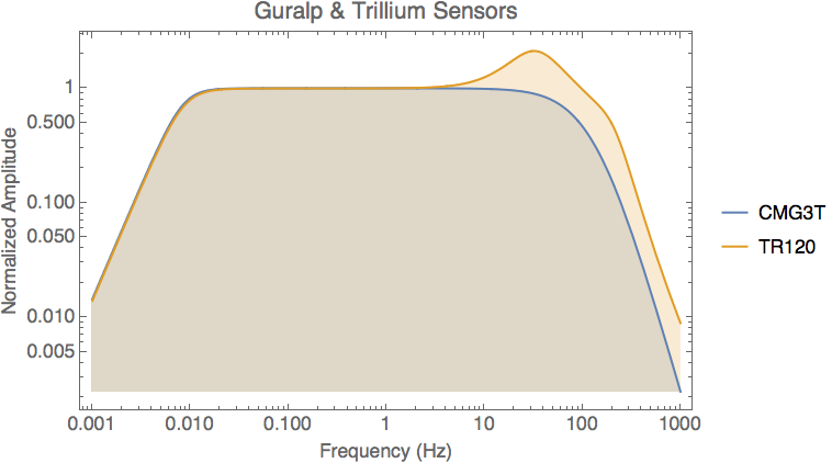
A comparison of the Guralp-3T and Trillium-120 amplitude response curves. The responses are normalized at 1Hz.