Compiled for the Penn State Geosciences Field Camp by Roman DiBiase and Erin DiMaggio.
**Note: This tutorial is loosely based on previous write-ups by Rudy Slingerland, Scott Miller, and Mike Oskin. Included in this document are links to the ESRI-USGS Geologic Mapping Template, the FGDC Digital Cartographic Standard for Geologic Map Symbolization, and the Geologic Cross Section Toolbox developed by Evan Thoms at USGS.
Table of contents
1.1 Loading base maps into ArcGIS
1.2 Downloading the ESRI Geologic Mapping Template
1.3 Projecting the Geologic Mapping database
1.4 Managing feature classes and topology in ArcCatalog
1.5 Adding the Geologic Mapping database to ArcMap
Section 2. Adding field data to your map
2.1 Adding XY data
2.2 Adding GPS data to your map
2.3 Georeferencing scanned field maps
3.1 Snapping
3.2 Editing lines
3.3 Editing points
3.4 Constructing polygons
Section 4. Making a geologic cross section
4.1 Installing the Cross Section Tools toolbox
4.2 Creating a new data frame
4.3 Extracting a segmented surface profile
4.4 Projecting point and line features into the cross section
4.5 Mapping in cross section
4.6 Annotating the cross section
5.1 The layout window and basic page design
5.2 Adding a legend
5.3 Adding a north arrow and scale bars
5.4 Adding text annotation
5.5 Exporting your map to PDF
Section 1. Getting started
For this section, you will set up your mapping document as well as the database structure for your geologic map that will be used for the remainder of the mapping exercise. We will be following the USGS style guide for making geologic maps. This is important so that the symbology for field observations and the communication of uncertainty is consistent when looking at maps produced by different authors. You will download the ESRI geologic mapping geodatabase and style sheet that contains all potential point, line, and polygon styles used for creating geologic maps, as well as appropriate labeling styles. We will be customizing this database to fit the goals of our mapping project.
You have also been provided with a document USGS_GeoMap_Symbols.pdf that describes in detail the numerous mapping points, lines, and polygons you will be using, and will be an important resource to keep handy. It is easiest to use the provided bookmarks to aid in navigating the 200+ page tome. If you are unfamiliar with the theory behind geologic mapping, or for example need a refresher on the difference between approximate and inferred contacts, it will be well worth your time to read the introductory material associated with the above document.
1.1 Loading base maps into ArcGIS
Open ArcMap and create a new “mxd” file. Load any basemaps (i.e., topographic maps, digital elevation models, satellite imagery) into your data frame, and set your project file geodatabase to be the default geodatabase. Navigate to \\File\Map Document Properties and select “store relative path names to data sources” (remember, your mxd file is simply a shell that points to the underlying data sets – if you change computers, or move your folders to a different location, you must keep the internal file structure consistent or risk having to manually reconnect the mxd file with the dataset locations). Once you have done this, save your mxd file and exit ArcMap.
**Note that if you are unfamiliar with ArcGIS, or need help downloading and processing your own basemaps, see Tutorial 1 and/or Tutorial 2. It is assumed here that you have already created or have been given the appropriate basemaps (link to project data for Geosc 497C).
1.2 Downloading the ESRI Geologic Mapping Template
If it was not provided you by your instructor, go to the website: http://arcscripts.esri.com/details.asp?dbid=16317 and download the 13MB file “ESRI_Geologic_Mapping_Template_1.2.zip” (Fig. 1). **Note that it will download to your computer as “AS16317.zip”.

Figure 1. Geologic Mapping Template download.
Extract the folders “ESRI_Geology.gdb” and “Fonts and Styles” to your work directory (Fig. 2).

Figure 2. Contents of the downloaded zip file, with key folders highlighted.
1.3 Projecting the Geologic Mapping database
For the next few sections, we will be working within ArcCatalog, a companion program to ArcMap that is used for managing file and geodatabase properties. Open ArcCatalog from the Start Menu and navigate to the file geodatabase “ESRI_Geology.gdb” in your project folder (Fig. 3). You may need to Connect to Folder if you do not see the path in the Catalog Tree.

Figure 3. ArcCatalog layout, showing blank mapping geodatabase downloaded in Section 1.2 above.
Next, we need to add the custom toolbox “GMT_Tools” to ArcToolbox. These are a series of Python scripts that automate tasks such as projecting multiple feature classes at once. Open the ArcToolbox window if it is not open already (Fig. 3), and then right click in the blank space at the bottom of the window, select Add Toolbox, and navigate to and open “GMT_Tools” (Fig. 4). This will add a folder to your ArcToolbox called Geologic Mapping Tools.

Figure 4. Add Toolbox dialog box.
Annoyingly, there is a minor bug in the downloaded toolbox that needs to be fixed. Right click the tool \\Geologic Mapping Tools\(2) Apply Coordinate System to ESRI_Geology.gdb, and select Edit to bring up model flow chart (Fig. 5). Here, simply click the Save button on the toolbar or go to \\Model\Save, and then close the window. Any red “x” that was on the tool should be gone now in ArcToolbox.

Figure 5. Model flowchart for “Apply Coordinate System” tool.
Now we are ready to run the projection tool. Double click on \\Geologic Mapping Tools\(2) Apply Coordinate System to ESRI_Geology.gdb and enter the following parameters: for Project Geodatabase Location, navigate to your class folder; for Project Geodatabase Name, type “Mapping_database”; for Project Coordinate System, choose the UTM coordinate system appropriate for our map (for Geosc 497c, this is: \\Projected Coordinate Systems\UTM\WGS 1984\Northern Hemisphere\WGS 1984 UTM Zone 44N), and leave the other fields unchanged (Fig. 6). It may take a while for the tool to run (~3 minutes on my laptop), but when it is finished you will have a new, appropriately projected geodatabase for your mapping. At this point you can delete the geodatabase “ESRI_Geology.gdb” for clarity. **Note that you may have to close ArcCatalog and delete the folder in Windows Explorer.
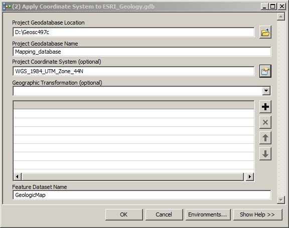
Figure 6. Apply coordinate system to ESRI_Geology.gdb tool dialog box.
1.4 Managing feature classes and topology in ArcCatalog
Before we can start mapping, we will need to customize a few components of the feature dataset “GeologicMap” to our project.
First, we will populate the feature class “MapUnitPolys” with the appropriate geologic units. Right click on the feature class “MapUnitPolys” and open the Properties dialog box (Fig. 7). In the Subtypes tab, select the Subtype Field “MapUnitDesc_ID”, and populate the Subtypes in stratigraphic order with the appropriate geologic units, and press OK to finish. For Geosc 497c, use the following: 0. undefined; 1. Salt Flat; 2. Alluvium (young); 3. Alluvium (old); 4. Mesozoic-Neogene; 5. Carboniferous-Permian; 6. Silurian-Devonian; 7. Cambrian.

Figure 7. Adding geologic mapping units to the Subtypes in Feature Class Properties.
Next, we need to add two line feature classes: the boundary of our map, and cross section lines. Right click in a blank area within the feature dataset “GeologicMap” (below “VolcanicPointFeatures” is easiest), and select \\New\Feature Class. Name the feature class “MapBorders”, change the Type to “Line Features”, and click Next – Next – Finish keeping all the remaining parameters as is (Fig. 8).

Figure 8. New Feature Class dialog box for creating MapBorders.
To add the cross section line, do the same thing, but this time Name the feature class “XSections” (also a line feature), and in the last dialog box, add a Field Name called “SectionID” of Data Type “Text” (Fig. 9), and press Finish.
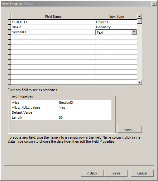
Figure 9. Adding a data field to the cross section line feature class.
Finally, we need to define the topology for our mapping feature dataset, which sets the rules for how features are allowed to interact with each other.
As above, right click in a blank space and select New\Topology. Name the topology “GeologicMap_Topology”, enter a cluster tolerance of 0.001 Meters, and click Next (Fig. 10).

Figure 10. Creating a new topology.
Next, select the feature classes “Contacts”, “Faults”, “MapBorders”, and “MapUnitPolys” to participate in the topology, and click Next twice. Now, we need to specify some rules for how these feature classes can interact, in order to minimize issues with constructing polygons for our geologic map (Fig. 11).

Figure 11. Adding a rule for feature class topology.
You will add the following rules: “Contacts” must not intersect; “Faults” must not intersect; and “MapBorders” must not intersect and must not have dangles (Fig. 12). Once you have done this, click finish and do not validate the topology if asked (you should not have any features yet). Close ArcCatalog when you are finished.

Figure 12. Topology rules used for the feature dataset “GeologicMap”.
1.5 Adding the Geologic Mapping database to ArcMap
Now we are ready to add our dataset to ArcMap and begin mapping by editing the appropriate feature classes. First, open the mxd file you created in Section 1.1. Add the feature dataset “GeologicMap” to your table of contents, and then right-click and group all of the items together to help in navigation (Name the group something like “Mapping”). You will notice a large number of potential mapping symbols in the table of contents. You will not use all of these! The attached PDF “USGS_GeoMap_Symbols.pdf” has descriptions to go along the unit codes (i.e., 1.1.1 Contact—Identity and existence certain, location accurate). To ease the clutter, you can remove layers that you will not be using. You can always add a layer later if you decide you need it (Fig. 13).
Finally, change the symbology for the feature class “MapUnitPolys” to the desired color scheme. For Geosc 497C, we will use the following CMYK color values (C%.M%.Y%.K%): Salt flats – 0.0.0.0; Alluvium (young) – 0.0.30.0; Alluvium (old) – 0.0.50.0; Mesozoic-Neogene – 8.30.70.0; 5. Carboniferous-Permian – 50.0.13.0; Silurian-Devonian – 40.40.0.0; 7. Cambrian – 8.30.30.0.

Figure 13. Organized table of contents.
Section 2. Adding field data to your map
In this section, you will learn how to add field observations and data to your map in the form of XY tables (Section 2.1), GPS data files (Section 2.2), and scanned field maps (Section 2.3).
2.1 Adding XY data
To aid in your mapping, you have been provided with an excel spreadsheet containing GPS observations from the field, including strike and dip measurements of bedding and contact attitudes. In this section we will import these measurements into ArcGIS.
Open the spreadsheet field_observations.xlsx. Here you will see your Easting (X) and Northing (Y) measurements (this is what you will be reading from your GPS in the field), the strike and dip measured at that location, and any additional notes. Not all points have strike and dip measurements – some are simply observations of a contact or geologic unit.
To import these data into ArcMAP, navigate to and open \\File\Add Data\Add XY Data… (Fig. 14). In the “Choose a table…” area click on the Folder Icon and navigate to where you have your XY data spreadsheet located. Double click on the excel file, then select the worksheet that contains the data. In the X Field, use the drop down menu to select “Easting” (your UTM Easting measurement) and in the Y Field select “Northing” (your UTM Northing measurement). Leave the Z field blank. Be sure the coordinate system matches your map (For Geosc 497C, WGS 1984 UTM Zone 44N) and click “OK” at the bottom. Click OK for the warning that may come up, and you will see the points on your map.

Figure 14. Adding XY Data Window.
You can save these points permanently to a feature class by right clicking the layer and selecting Export Data, choosing your project geodatabase as the file location, and saving as type “File and Personal Geodatabase feature classes”, with a name like “Field Observations”.
It will help to label the features with the strike and dip for when you add bedding attitudes to your map (Section 3.3). To do this, double click on the feature class “Field Observations”, and navigate to the Labels tab (Fig. 15).

Figure 15. Labels tab of the Layer Properties window.
Be sure to check the box that says “Label features in this layer”, and then click the box “Expression” to open a new window that enables combining values from different fields (in this case Strike and Dip) into a single label. You will need to use the VBScript parser to combine the [strike] and [dip] fields with a comma string (Fig. 16).
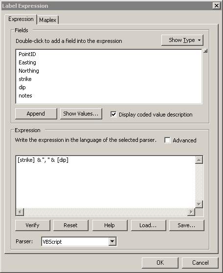
Figure 16. Building an expression for labeling features using multiple fields.
Click “Verify” to make sure you typed the code in correctly, and then click okay. You should now see all of your points labeled with “strike, dip” (Fig. 17).

Figure 17. Screenshot of map showing “Field Observations” feature class labeled with strike and dip.
*Note that if you find it hard to read your labels and symbols, you can right click on the Data Frame and select “Set Reference Scale” to fix the scale relative to the map. However, be sure that you clear the reference scale before printing your map.
2.2 Adding GPS data to your map
To add waypoints and tracks from a handheld GPS, use the tool \\Conversion Tools\From GPS\GPX To Features. It should be self-explanatory.

Figure 18. GPX to Features dialog box.
2.3 Georeferencing scanned field maps
Section 3. Editing your map
In this section you will learn how to edit the feature classes within your mapping geodatabase to construct a professional looking geologic map with appropriate annotations and labeling.
3.1 Snapping
Open the Snapping Window (Fig. 19) by selecting “Editor” then with your mouse on “Snapping” select “Options”. Snapping occurs when you are editing and your mouse gets close to another line that you have created. You can set a “Tolerance” so that when you get within a specified number of pixels from another line, your mouse will “SNAP” or move to follow directly one that other line. The benefit of this is that it allows you to easily prevent dangles while editing. However, there is a fine line between having the tolerance too high (say 30 pixels) and too low (say 1 pixel), all of which will depend on the scale at which you are mapping. For this project you will probably want to use the default tolerance (5 pixels) or possibly increase it to 10 or more pixels. Play around with what you find best.

Figure 19. Snapping Options Window.
3.2 Editing lines
3.2.1: Editing feature class: MapBorders
Although we have already provided you with a feature class of your map border, we want to re-trace it make it part of your mapping geodatabase (so that all of your data is one place). To start add the feature class “mapping_extent” we provided to ArcMap and start editing the feature class “MapBorders” within your mapping geodatabase by selecting \\Editor\Start Editing from the Editor toolbar menu. **Note that this is a bit confusing – sorry! It will be useful to keep the feature class “mapping_extent” handy for clipping your map – we will be using the feature class “MapBorders” for the cross section as well, so it won’t be useful as a clipping layer.
In ArcMap make sure the Create Features window is open. If not, navigate to the Editor toolbar menu and select \\Editor\Editing Windows\Create Features and the window will open (Fig. 20).

Figure 20. Editing MapBorders feature class.
When you select the feature class “MapBorders” with your cursor, the Construction Tools window will appear at the bottom of the same frame (Fig. 21). In this case we want to draw four separate lines that define the extent of our mapping area, so select Line. Make sure the feature class “mapping_extent” is visible, so you can trace it precisely by snapping to the vertices. You should now have created a new rectangle that covers your mapping area. Go to the editing toolbar and select \\Editor\Save Edits. Remember to save your edits early and often!!

Figure 21. Construction Tools for creating lines.
3.2.2: Editing feature class: Xsections
Similar to above, create a cross section line, or trace the provided cross section(s) by editing the feature class “Xsections”. Be sure to provide a name for the cross section in the field “SectionID” of the attribute table using the format “XS1”, “XS2”, etc.
3.2.3: Editing feature class: Contacts
First, open up the PDF “USGS_GeoMap_Symbols.pdf” that you received last week that contains descriptions to go along the unit codes for your mapping. View the bookmarks on the left side for easy navigation. You will mainly be using the following 4 line types: Accurate | Approximate | Inferred | Concealed. If you have forgotten what these line types mean, review the intro material provided in this PDF.
In ArcMap, select (check) the layer “Contacts” in your Table of Contents and start editing the feature class “Contacts”. You should now see many different line types for representing contacts (the same as those in your PDF, each of which are numbered) in the Create Features window (Fig. 22). Looking at the USGS_GeoMap_Symbols.pdf, determine the numbers of the 4 highlighted contacts that you will be using. In this case they are (1.1.1 = Accurate | 1.1.3 = Approximate | 1.1.5 = Inferred | 1.1.7 Concealed).

Figure 22. Create Features window for “Contacts” feature class. (note only showing a portion of the features).
Select the line type that you would like to start with (say, 1.1.1 accurate). In the Construction Tools window (Fig. 21) select Line and begin editing.
Some pointers while editing:
– To finish a line, double click on the last point
– You can edit just one of the vertices be using the arrow tool in your editing tool bar, selecting the line by double clicking on it, and using the “Edit Vertices” tool bar that opens up (Fig. 23). You can move vertices (arrow button) add vertices (plus) and delete vertices (subtract).

Figure 23. Edit Vertices window
– You will be spending A LOT OF TIME CREATING LINES. One of the MOST IMPORTANT things to remember about creating lines is that all of your contact lines should follow the topology described in Section 1.4, and finish at either a contact or a fault (no dangling contacts!). Additionally, when mapping an enclosed unit, the topology does not like a single line feature to close on itself. Use the Split tool on the editor toolbar, or draw two separate lines to close the loop.
3.2.4: Editing feature class: Faults
Follow the same method for editing above. Some of the boundaries between geologic units will be fault lines, but not all fault lines need be contacts (i.e., sometimes it is easiest to draw contacts first, and then add the faults afterward). Refer to the USGS PDF to see the highlighted fault types that you will be using (Fault, Normal Fault, Reverse Fault, and Strike Slip). Note that there is a directionality to your lines that determines which side line decorations (e.g., thrust barbs) fall on. This directionality can be switched by right clicking on the line feature class while in edit vertices mode (Fig. 23), and selecting flip.
3.2.5: Editing feature class: Folds
Follow the same method for editing above, however folds are NOT contacts and therefore they will not follow the same topology. This means that you will simply add fold lines to your map that may intersect contact or fault lines.
3.3 Editing points
3.3.1: Adding bedding measurements to your geologic map
Although we have loaded our field observations into our map, they do not have the appropriate symbology or labeling format. To fix this, we need to edit the point feature class “Bedding” within our mapping geodatabase.
First, we need to set up the symbol rotation and labeling. Before starting, make sure to stop your editing session by selecting \\Editor\Stop Editing from the Editor toolbar menu. Right click on the feature class “Bedding”, and go to the Symbology tab (Fig. 24). Make sure that the checkbox “Clockwise” is checked, otherwise your strike and dip symbols will be turned the wrong way. **Note that this box will be greyed out if you have an editing session open.

Figure 24. Representations window of the Symbology tab.
Next, click the blue cylinder at the bottom right labeled “Display field overrides”, and set the Angle to the “Azimuth” field (Fig. 24). This will force the rotation of the symbol to the strike azimuth you define, and save you an extra step of typing in the symbol rotation.
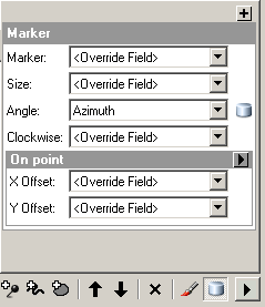
Figure 25. Display field overrides window.
To appropriately label features, enable the Labeling toolbar (Fig. 26) if it is not already enabled (//Customize/Toolbars/Labeling), and select “Use Maplex Label Engine”.
Figure 26. Labeling Toolbar.
Next, click the Label Manager button to bring up the Label Manager window. Select “Default” below the “Bedding” feature class, set the Label Field to “inclination or dip”, and click the Label Styles button (Fig. 27).

Figure 27. Label Manager window.
In the Label Style Selector window, go to More Styles, and choose “Geology_Template”. If you do not see this option, select “Add…” and navigate to “Geology_Template.style”, which should be in the “Fonts and Styles” folder you downloaded from ESRI. Once added, navigate to the style “Orientation point”, and select OK (Fig. 28).

Figure 28. Label Style Selector window.
Last, from the Label Manager window (Fig. 27), click “Properties…” and click the options box next to Rotate by Attribute. Here, choose “Azimuth” as the Rotation Field, and then change the Additional Rotation to 90 (Fig. 29). This will orient the label appropriately next to the tick mark on the bedding symbol.

Figure 29. Label rotation window.
Now, we are finally ready to start editing. Start an editing session, and bring up the Create Features dialog box (Fig. 30). Navigate to the feature class “Bedding” and the feature representation 6.2. **Note that the Bedding feature class must be visible in your table of contents to show up in the feature templates.

Figure 30. Create Features dialog box showing Bedding representation.
You should still have Snapping on (Section 3.1), so it should be straightforward to add a point directly on top of your feature class “Field Observations” at the points with strike and dip measurements. After creating a point, select the Attributes tab from the either the Editor toolbar or the Create Features window (Fig. 30). Here, type in the appropriate strike and dip values for the fields “Azimuth or strike” and “Inclination or dip” (Fig. 31).

Figure 31. Attributes window, showing editing of strike and dip fields in the feature class “Bedding”.
Do this for all the strike and dip measurements on your map, and then turn off the feature class “Field Observations” to reveal nicely labeled and rotated bedding attitude symbols (Fig. 32).

Figure 32. Appropriately labeled strike and dip symbol (compare to Fig. 17)
3.3.2: Adding fault and fold ornamentation points
Often times you will want to indicate the sense of slip on faults, or indicate fold geometry. We will do this by adding points manually to our map from the feature class “ObservationsOrnamentations_Faults” or “SmallMinorFolds” (Fig. 34). **Note that there is no ornamentation layer specifically for folds – this is probably a mistake on ESRI’s fault, but nonetheless we can get the desired effect using the ornamentation provided in “SmallMinorFolds”.

Figure 33. Fault and fold ornamentation feature classes.
Note that you will have to rotate these symbols manually (i.e., by eye), using the representation editor in the attributes window (Fig. 34, Fig. 35).

Figure 34. Intial, unrotated, placement of fold ornamentation (anticline symbol).

Figure 35. Properly rotated fold ornamentation.
3.4 Constructing polygons
Once we have gotten most of our linework done, it is time to start filling in the areas with polygons.
First, open the Topology toolbar, and validate the topology in the current extent (Fig. 36). Error will appear as red highlights on your map. Take the time to fix these according to the rules described in Section 1.4 before moving on.

Figure 36. Topology toolbar showing validate topology button.
Next, in order to construct a mapping polygon using the existing linework, select the boundaries of the polygon you wish to map using the Edit Tool (arrow) on the Editor toolbar (Fig. 37). To select multiple lines, hold the shift key. As you progress, it is unavoidable that you will select polygons as well. You can deselect the polygon features by selecting somewhere in their interior.

Figure 37. Selecting boundaries for mapping polygon.
Once you have selected a properly enclosed (i.e., no gaps) set of bounding lines, use the “wrench” tool on the Advanced Editing toolbar (Fig. 38) to open the Construct Polygons dialog box (Fig. .
Figure 38. Advanced editing toolbar.
Choose the appropriate template, and then click OK (Fig. 39).

Figure 39. Construct polygons dialog box.
Occasionally, you will generate multiple, overlapping polygons due to the nature of your linework. This is unavoidable in some circumstances, and requires deleting unnecessary polygons after the fact.
If you make a mistake, or change your mind on the location of a contact, you can edit the linework and polygons concurrently using the Topology Edit and Modify Edge tools on the Topology toolbar. You can see which features are shared by opening the Shared Features window from the Topology toolbar. After clicking Topology Edit (second button from the left), select the boundary you wish to modify (it will turn magenta). Next, click Modify Edge, and adjust the boundary using the Edit Vertices toolbar (Fig. 23, Fig. 40). When finished click anywhere on the map to complete the changes (Fig. 41).

Figure 40. Topology editing of shared feature.

Figure 41. Finished modification of shared feature.
Section 4. Making a geologic cross section
Traditionally, geologic cross sections have been drafted either by hand, or using vector drawing programs such as Adobe Illustrator or Inkscape. This often requires tracing or exporting topographic profiles, determining locations of contacts and faults along the cross section, and projecting strike and dip measurements into the plane of the cross section (being careful to calculate apparent dips). All while being faithful to the vertical exaggeration typically needed to communicate the interaction between topography and geologic structure.
For this course, we will be using a series of Python scripts developed for ArcGIS by Evan Thoms at the USGS (https://github.com/evanthoms/Cross-Section). These tools automatically extract the surface expression of your geologic map along a topographic profile, including the appropriate projection of nearby bedding measurements and vertical exaggeration. The actual cross section occupies a corner of your map, centered on 0,0, which allows you to draw contacts, faults, ornamentation, and construct polygons all using the same mapping symbology as your geologic map.
While ArcGIS is hardly the ideal environment for drafting and annotating figures, for the scope of this class we will be doing everything within one program. If you are more comfortable using Adobe Illustrator, Inkscape, or Microsoft Powerpoint, you can export the cross section and annotate it elsewhere.
4.1 Installing the Cross Section Tools toolbox
If you have not already been provided with the Cross Section toolbox and scripts, download the 61MB file “Cross-section-master.zip” from the above URL and extract the file to your project folder.
Similar to what we did previously (Section 1.3), open your map in ArcMap and add the custom toolbox “Cross Section Tools” to ArcToolbox. You should see a number of scripts show up (Fig. 42).

Figure 42. Cross Section Toolbox.
Before moving on, it is important to note that none of the following will work if your map is not in a projected coordinate system with the same horizontal and elevation units (e.g., UTM). If you have been following along, you should be fine.
4.2 Creating a new data frame
Rather than start a new mapping project, you will create a new data frame in which to work on your cross section. From the main menu, navigate to and select \\insert\data frame. It may be helpful to rename your original data frame from the default “Layers” to “Geologic Map”, and the new (empty) data frame to “Cross Sections” in the data frame properties dialog box.
Next, we want to populate the new data frame with your digital elevation model and your mapping layers (i.e., Xsections, Bedding, Contacts, Faults, Fault Ornamentation, MapUnitPolys, and MapBorders). This is most easily done by dragging and dropping each individual layer from the original data frame to the new data frame (Fig. 43). You can also add the data through the catalog window, but this requires redefining the symbology for the layer MapUnitPolys, which is tedious. To switch back and forth between data frames, right click on the data frame you wish to use and select Activate. Both of these data frames will show up in Layout View as separate objects, allowing you to put both your map and cross section on a single page.

Figure 43. Table of Contents showing two data frames – one each for the map and cross section.
4.3 Extracting a segmented surface profile
The first step in generating any cross section is to extract a topographic profile along the cross section line. If you have not already done so, open an editing session and create your cross section line using the feature class “Xsections”, and type in a name such as “XS1” in the “SectionID” field of the attribute table (Section 3.2.2).
Before starting, make sure that the data frame “Cross Section” is the active data frame (it should be bold), otherwise activated it as described in Section 4.2. Also be sure all editing sessions in both data frames are closed. To extract a segmented surface profile, navigate to and run the script \\Cross Section Tools 10.2\Create Segmented Surface Profile from ArcToolbox (Fig. 44). Enter in your cross section line layer (“Xsections”), DEM layer, and geology polygon layer (“MapUnitPolys”). For most cases it is fine to start the line from the northwest. The output feature class should be saved to your mapping geodatabase with a name like “xs1_segmented_profile”, and added to the data frame “Cross Sections” (assuming you renamed your new data frame as described in Section 4.2).
The ideal vertical exaggeration will vary depending on location. For the mapping project in Geosc 497, use a vertical exaggeration of 2.

Figure 44. Create segmented surface profile dialog box.
Once you have entered all the parameters, click OK to generate a topographic profile segmented according to the surface geology you mapped. To see your profile, you will need to right click on the feature class “xs1_segmented_profile” and select Zoom To Layer.
For the purposes of mapping, it is helpful to modify the line symbology to match the colors on your geologic map according to the map unit number (Fig. 45, Fig. 46). You may need to open up the feature class “MapUnitPolys” to remember the connection between the numeric “MapUnitDesc_ID” field and the actual unit names.
**Note that when you finalize your cross section, it is important to return the symbology to a uniform thin black line (0.5 thickness).

Figure 45. Changing symbology of segmented surface profile.

Figure 46. Segmented profile colored by geologic unit.
4.4 Projecting point and line features onto the cross section
In this step, we will use the Cross Section toolbox to project our strike and dip measurements into our cross section, and locate the position of any faults present. However, in order to do this, we need to populate the “Symbol Rotation” field in the feature class “Bedding” with values of dip direction (strike azimuth + 90° using the right-hand rule).
Open the attribute table for the feature class “Bedding”, right click on the field heading “Symbol Rotation”, and select Field Calculator. Click yes when asked to make a calculation outside of an edit session.
In the Field Calculator, type “[Azimuth] + 90” and click OK (Fig. 47). This should populate the field “Symbol Rotation” with the appropriate values for dip direction.
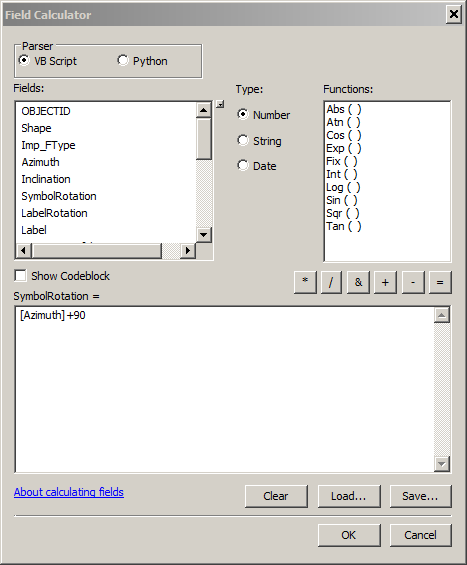
Figure 47. Using Field Calculator to create a column of dip direction values.
Now we are ready to create some tadpoles. Navigate to and open the tool \\Cross Section Tools\Map points to cross-section points from ArcToolbox (Fig. 48). Here, enter the same layers and values from above (Fig. 44), paying particular attention to using the same values for “Begin measuring line from” and “Vertical exaggeration”. For the points layer, use the feature class “bedding”; for the azimuth field, use the field “SymbolRotation”; and for the dip field, use the field “Inclination”.
For the search distance, it is important to choose a value that is large enough to capture all of the appropriate bedding attitudes, but small enough so that you are not incorporating values from structures not represented in your cross section. For the mapping project in Geosc 497, a good value for the search distance is 7 kilometers.
Name your output file something like “xs1_map_points” and add it to the data frame “Cross Sections” as above. Click OK, and you should see a number of “tadpoles” that indicate the apparent dip from each of the strike and dip measurements projected into the cross section plane and with the appropriate vertical exaggeration (Fig. 49).

Figure 48. Map points to cross-section points dialog box.

Figure 49. “Tadpoles” showing bedding attitude.
Next, we want to do the same thing for any faults that intersect our cross section line. Navigate to and open the tool \\Cross Section Tools\Line intersections to cross-section features from ArcToolbox (Fig. 50). Again, use the same values for all fields, except this time use the feature class “Faults” and name the output file something like “xs1_fault_intersections”. You can either choose to have the intersections characterized with a thin line (Fig. 51), or a point (whichever you like).

Figure 50. Line intersections to cross-section features dialog box.

Figure 51. Segmented surface profile showing bedding measurements and fault intersection.
4.5 Mapping in cross section
Now we are set to start mapping. First draw a box around your cross section using the feature class “MapBorders”, being mindful not to make your cross section excessively deep (1-2 km max). Then start extending your surface units to the subsurface, using the tadpoles as a guide (Fig. 51). Create contacts and faults in the subsurface, and when you are finished, construct polygons in the same way as you did for your geologic map in Section 3.4. Last, be sure to change the symbology of the surface profile to a thin (0.5 pt) black line (Fig. 52).

Figure 52. Cross section with constructed polygons and fault annotation.
4.6 Annotating the cross section
Annotating your cross section is somewhat tedious, but doable, in ArcMap. It is also acceptable, but not necessary, to export to Illustrator or Inkscape to finalize your figures. The key components that need to be added are the cross section labels and directional indications, distance and elevation tick marks, and an indication of vertical exaggeration.
To add distance and elevation marks, it is helpful to use the Drawing toolbar in Layout mode. Conveniently, the coordinates shown at the bottom right of the window follow along with your cursor, and indicate the relative distance and elevation along your profile. The distance values will be correct, but the elevation will be scaled by the vertical exaggeration; for example, if using a vertical exaggeration of 2x, a value of 4000 m will correspond to an elevation of 2000 m.
**Note: you can make your horizontal axis by inserting a scale bar and modifying the increments accordingly.
The final, annotated cross section should look something like Fig. 53.

Figure 53. Finished cross section showing appropriate annotation.
Section 5. Layout and design
The final stage of preparing a geologic map is to add a descriptive legend and all appropriate annotation (e.g., north arrow, scale bar, title, author). The best way to get a sense of what is needed is to look at geologic maps published by the USGS or state geological surveys (Fig. 54).

Figure 54. Pennsylvania Geological Survey bedrock geologic map of the McCoysville quadrangle, PA (external link). Note the brief descriptions of mapping units in stratigraphic order, the description of all symbols used on the map, and a geologic cross section with the same scale as the map.
While a bit clunky at times, it is possible to do all of the layout within the ArcMap program. In some cases it may be easier to make fine scale edits using an external vector drawing program, such as Adobe Illustrator or Inkscape.
5.1 The layout window and basic page design
We have mostly been working in “data view” for exploring our mapping area and editing our mapping geodatabase. In order to design our final map, display multiple data frames concurrently, and add a legend and annotation, it is necessary to switch to “layout view” by going to \\View\Layout View. If you have been following along, you should have two data frames shown in the map window – one for your geologic map, and one for your geologic cross section.
Depending on the detail and extent of your mapping, you will need to adjust the scale and size of your map, cross section, and map sheet (i.e. print size of the entire map). For the mapping area in 497, use a scale of 1:200,000 for BOTH your geologic map and your geologic cross section, by typing in “200,000” into the map scale box on the Standard toolbar (Fig. 55).
Figure 55. Standard toolbar showing map scale.
Next, adjust the page layout by going to \\File\Page and Print Setup and changing the width and height of your map page to 17” x 11” (Fig. 56). This should provide plenty of room to add a detailed legend and annotation.

Figure 56. Page and Print Setup dialog box.
After you have adjusted the scale and page dimensions, drag the extent of the Data Frames to show the full extent of your mapping area and cross section. It makes things much easier if you go to the Data Frame properties for your geologic map and enable “clip to shape” using the feature class Mapping Extent (Fig. 57). **Note that this is not the line feature class MapBorders in your mapping geodatabase, but the original polygon feature class I provided. Clipping to the extent of MapBorders will not work because the feature class encompasses your cross section as well.
To retain a nice looking border to your map, be sure to click Exclude Layers and exclude the feature class MapBorders from the clipping. For both of the data frames, it will keep things tidy to remove the default border for the data frame by changing the data frame border to “none” in the Frame tab of the Data Frame Properties window.

Figure 57. Data frame properties dialog box showing Clip Options.
5.2 Adding a legend
Adding a legend in ArcGIS is a multi-step process with lots of flexibility. Unfortunately, the default legends tend to be awful, and thus generating something presentable requires fine tuning using a pretty clunky interface. Before starting, be sure that you are generating your legend while the geologic map data frame is activated (rather than the cross section data frame). This will ensure that all of your mapping symbols will be available for the legend.
5.2.1 Adding map unit descriptions
First, you will add a short (less than 30 words or so) description to each of your map units. This is done through the Symbology tab of the Layer Properties window of the feature class MapUnitPolys. Here you should see your mapping units listed in stratigraphic order (youngest at the top), with their corresponding symbol (color), value (e.g., 1, 2…), and Label (e.g., “Cambrian”). For each unit, right click on the label and select Edit Description (Fig. 58). This will bring up a dialog box where you can type or paste the description you wish to include. **Note that the only place where this description will be visible is in the legend!

Figure 58. Edit description option in the Symbology tab of the Layer Properties dialog box.
While you are at it, change the heading label from “MapUnitDesc_ID” to something more useful, like “Geologic mapping units” or “Map unit explanation”.
5.2.2 Generating a legend for the feature class MapUnitPolys
Rather than build a single, all-inclusive legend, it is often more straightforward to separate out major groups of legend items into multiple legends. The first legend to build is that for your geologic mapping units.
While in layout mode, navigate to and select //Insert/Legend. By default, all visible layers will be included as Legend Items. Use the single left arrow button to remove all layers except for MapUnitPolys, and click Next (Fig. 59).

Figure 59. Insert Legend dialog box – Legend Items.
In the next window, clear the text from the Legend Title box and click next (often times it is unnecessary to include the generic term “Legend” on your map (Fig. 60).

Figure 60. Insert Legend dialog box – Legend Title.
For the Legend Frame, choose no border, background or drop shadow (all default) and click next. For the patch size, choose the size and shape of the symbol used in the legend for each item. To see a preview of the size relative to your other map elements, click “preview”. A rectangular patch size of 40 x 40 pts. is a good place to start (Fig. 61). Click next, and then Finish to generate the legend.

Figure 61. Insert Legend dialog box – Patch Size.
Often the default text and/or layout of the legend is not optimal. To change this, right click on your newly created legend and select Properties to bring up the Legend Properties window. Here you can modify the Style of each of your legend items, to adjust the relative position and visibility of the patch, header, label, and description, as well as the font sizes (Fig. 62, Fig. 63).

Figure 62. Legend Item style selector.
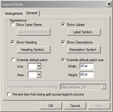
Figure 63. Legend Item style properties window.
5.2.3 Generating a legend for linework and points
The second legend you will build is one for all of your line and point work. Repeat the steps in Section 5.2.2, except this time include all the relevant feature classes you used in your mapping (e.g., Bedding, Contacts, Faults, Folds).
Initially, the legend will include dozens of representation types, most of which are not in use on any given map. To remedy this, right click on the legend to open up Legend Properties, and for each layer, check the box next to “Only show classes that are visible in the current map extent”.
In addition, you will want to rename each symbol with a more descriptive label than the default numeric code (e.g., 1.1.1). To change this, go to the Symbology tab in Layer Properties for each Layer, and change the label by double clicking on the existing label you wish to change (Fig. 64). You should see the changes in the Legend and Table of Contents as you do this.
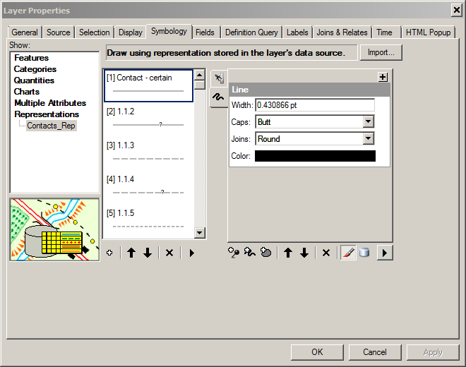
Figure 64.
Last, it is cleanest to remove all headings and layer names from this legend by appropriately adjusting the Legend Style for each layer (Fig. 63).
5.3 Adding a north arrow and scale bars
To add a north arrow, use \\Insert\North Arrow. This is pretty self-explanatory.
To add a scale bar for your map, use \\Insert\Scale Bar. Be sure to edit the units to metric (meters or kilometers depending on map extent), and adjust the number of divisions, subdivisions, and font size to be clear and legible.
Be sure to indicate both horizontal and vertical scale on your cross section. Ideally, the two will be at the same horizontal scale, so the same scale bar can work for both. Often it is helpful to include an axis for elevation, but this will need to be done manually using the drawing toolbar (see Section 4.6).
5.4 Adding text annotation
To add text annotation to your map (e.g., cross section directions/end points, vertical exaggeration…), use \\Insert\Text. If you want to “wrap” text (i.e., create a block of text), instead use the tool Rectangle Text from the Drawing toolbar.
Finally, be sure to add a title and your name to the map.
5.5 Exporting your map to pdf
To publish your map as a PDF file for sharing and printing, go to \\File\Export Map and save as type “PDF”. Be sure to to use 300 dpi resolution, and “best” image quality.