My paper on the radial velocity jitter of 600 planet-search stars – or as I call it “the big jitter paper” – was just recently published earlier this week and is now on arXiv! I’ve spent a lot of time over the last few years getting to this stage, so here’s a “brief” summary!
Intro:
In the search for low mass exoplanets, we are hampered by stellar variability, or “jitter,” that can drown out the signals of planets. The goal of this work is to better understand the astrophysical drivers of RV jitter and gain a broader picture of RV jitter for a wide range of stars. Let’s just jump right in to the take home plot:

There’s a lot to unpack in this plot, so I’ll go through it bit by bit. First let’s start with…
The Data:
The radial velocity measurements used in this work come from decades of Keck-HIRES observations (1-2 m/s single-measuremnt precision). In addition to the years’ worth of observations for each star, we also obtain simultaneous Calcium H&K measurements, SHK, that monitor the star’s magnetic activity level. We start with the entire sample of stellar properties from the Brewer et al. 2016 spectroscopic analysis, selecting those with surface gravities, log(g), that are consistent between their two methods. Now that we know where the data come from, it’s time to discuss how we went about measuring the RV jitter from the RV timeseries (the y-axis in the above plot)…
Measuring Jitter:
The goal is to isolate only the intrinsic stellar variability and remove anything else in the RV’s (i.e., companions!). Ironically, this is the exact opposite approach to planet-hunting, which is why “jitter” is often referred to as “noise” in the exoplanet community (I was even called out by the referee for calling it ‘noise’ in a few places). To isolate the stellar jitter I first searched for which stars had published planets and refit the planets by using the published values as input starting guesses; the remaining stars were all fit with a blind Keplerian fit. Following that, I went through each star diagnosing the fit, rejecting poor fits and adding in more planets when necessary. This vetting process, which we began calling “the slog,” was a laborious process that required multiple passes for most stars because it took into account: possible correlated activity from the activity timeseries (which we don’t want to remove!), data before and after the Keck-HIRES upgrades in 2004, outliers, stellar binaries and other long term linear trends. Once everything was subtracted out of the velocity timeseries that isn’t intrinsic stellar signal, we simply take an RMS of the residuals to calculate the RV jitter. With all that out of the way it’s time to discuss the results…
Results Part I: Two Regimes of RV Jitter and the “Jitter Minimum”
Let’s take another good look at this plot, which shows the RV jitter for our entire sample
The data points in the plot above form a strong overall ‘L’ shape: a vertical pileup of more yellow-orange color-coded stars and a mostly horizontal floor of purple-black color-coded stars. For the most part stars fall into one of these two regimes. We have long known that “jitter” and magnetic activity are correlated (spots, faculae, flares, etc.) and so the vertical branch of the ‘L’ is therefore clearly the young, active, main sequence stars still undergoing stellar spin-down. The horizontal floor has a slight rise to it, and so it cannot be explained purely by activity (which is still decreasing as the star evolves to the subgiant and giant regimes). Rather, the rise in the floor comes from convection: as a star evolves, its convective power increases and the amplitudes of both stellar oscillations and stellar granulation increase, which dominate the stellar jitter.
We have therefore empirically identified two regimes of RV jitter: activity-dominated and convection-dominated. Further, we can trace the jitter evolution of a typical star in this plot: it starts out at the top of the ‘L’ and decreases in jitter as it spins down on the main sequence. While still on the main sequence, it spins down enough that convection becomes the dominant component and it transitions from activity-dominated to convection-dominated and gradually increases in jitter as it evolves off the main sequence and into the subgiant and giant regimes.
This astrophysical framework for the jitter evolution of a star – transitioning from activity-dominated to convection-dominated – gives rise to the idea of a “jitter minimum,” the point in a star’s life where its jitter is at its lowest. This must occur during the transition from activity-dominated to convection-dominated, so it is very important for those who want to select the lowest jitter stars to know when this transition occurs for different types of stars. This brings us to…
Results Part II: The Mass Dependence of the “Jitter Minimum”
The gallery below shows the same plot as above but for individual bins of mass.
[It automatically progresses through the images. If you wish to look at a specific mass bin hover over to stop it and then click the arrows to step forward or backward. Clicking the image will bring up a larger gallery window to view. The lowest mass bin contains the legend]


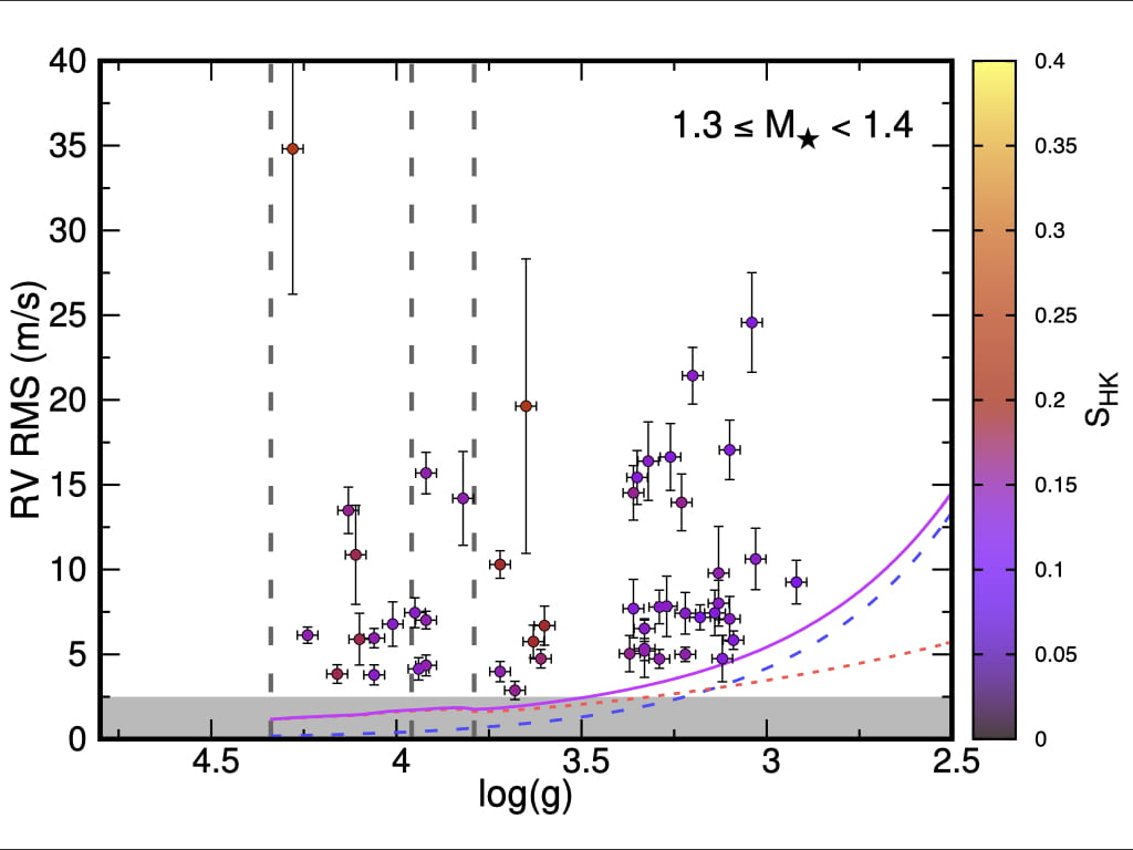
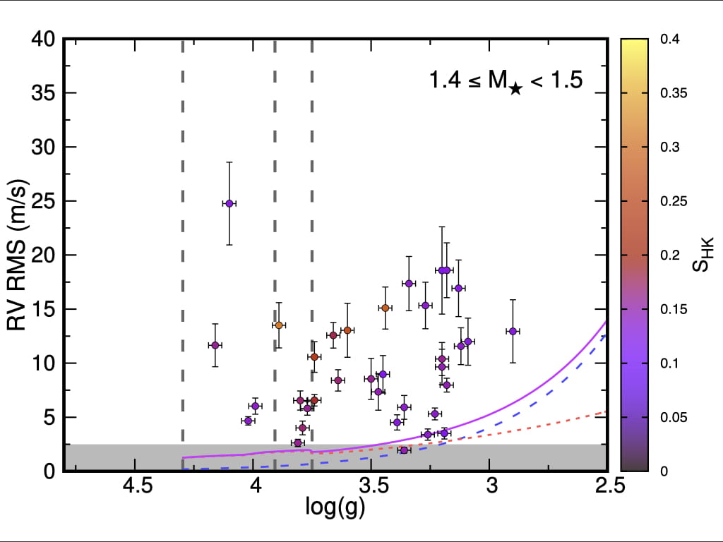


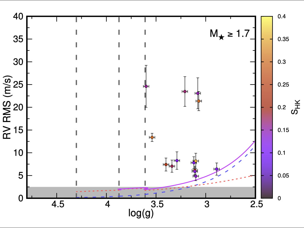
The above plots demonstrate how the jitter minimum changes with mass: As stars increase in mass, the jitter minimum occurs at later evolutionary stages! This makes sense, given stellar evolution: more massive stars evolve more quickly and so they spend much less time on the main sequence spinning down. As the masses increase, the ‘L’ shape becomes less and less sharp, tracing out a smoother transition and eventually becoming a mostly diagonal line for the highest mass stars in our sample. We therefore can break our sample into different types of jitter evolution depending on mass:
Low mass stars: drop vertically downward on these plots as they spin down on the main sequence. They have not had enough time in the age of the universe to evolve significantly on the main sequence and instead are largely activity-dominated. The stars in our sample reach the expected instrumental uncertainty level of about 2.5 m/s, so we are unable to say if they have actually reached their jitter minimum yet.
Solar-ish mass stars: follow the ‘L’ shape described in the previous section. For the lower mass stars that still show the full ‘L’ evolution, they drop nearly vertically and transition sharply to the convection-dominated regime. The higher mass stars in this group show the smoother, more gradual transition.
High mass stars: evolve so quickly that they are still spinning down as they leave the main sequence, resulting in a diagonal path downward and to the right. Compounding this effect is the fact that stars above the Kraft break (~1.3 solar masses) have very thin or nonexistent convective envelopes on the main sequence, which means they are unable to generate a magnetic dynamo and spin down through magnetic braking. As a result, for these highest mass stars in our sample, the spin-down (and the corresponding decrease in RV jitter during the activity-dominated regime) is delayed until they evolve into the subgiant regime and develop a thick enough convective envelope to generate a magnetic dynamo and spin down.
The image below shows a schematic of the jitter evolution for different masses of stars and illustrates the features highlighted above.

How Can We Use This?
- Test the Models: This sample gives us an empirical dataset to test our theoretical models. The earlier plots grouped by mass showed theoretical predictions for both the granulation and oscillation components from Kjeldsen & Bedding (2011), which showed relatively good agreement to our jitter floor. We also compared several other theoretical predictions (and some semi-empirical relations based on Kepler photometry) for these components before settling on this particular theoretical prediction. On the activity side of things, many groups are generating synthetic spectra in the presence of various magnetic activity effects such as spots and faculae to better understand how they affect RV measurements. Our large empirical sample across a wide range of stellar types make this a valuable sample for model comparisons here as well.
- Select and Prioritize Targets: With a better understanding of RV jitter and how the “jitter minimum” depends on mass, we can use this sample to estimate the expected amplitude and dominant components of RV jitter for a star across a wide range of stellar parameters. This will inform both target selection for RV surveys and prioritization for RV follow-up of planet candidates from transit surveys (e.g., TESS, CHEOPS, PLATO).
- Optimize Observing Strategies: Obviously, some targets are scientifically interesting enough to observe despite potentially having higher jitter. For these cases especially, it becomes important to know the expected dominant component so that the proper mitigation strategies can be implemented (observational and/or computational)
- Predicting Jitter: Similar to the above, this sample provides an excellent set for building a robust jitter predictor that starts with the astrophysical framework presented here and incorporates stellar uncertainties to allow for accurate jitter predictions. I’m working on finishing up this project so stay tuned for more…
Leave a Reply
You must be logged in to post a comment.