Advisors: Dr. Tess Russo (Department of Geoscience, Penn State), Dr. Ludmil Zikananov (Department of Mathematics, Penn State), Dr. Katherine Zipp (Department of Agricultural Economics, Sociology, and Education, Penn State)
Updated: December, 2016
Motivation:
 With changing climate and water resources, the world is faced with the challenge of balancing food security with sustainable water use. This issue is currently playing out in Punjab, India where the Green Revolution has enabled huge agricultural growth based on an unsustainable irrigation system. Rice, a water intensive crop, has increased from 7% of land use in 1970 to 50% of land use in 2001 (Takshi and Chopra 2004). Punjab provides 40 -50% of India’s rice and 60 -65% of India’s wheat (Aggarwal et al 2009). This large amount of agricultural production has lead to the overexploitation of groundwater resources, causing the water table is decreasing on average .4m/yr (Kahn et al 2007). Many solutions have been proposed but few rigorous quantitative analyses or simulations of proposed strategies have been done that consider both the economic and hydrologic components of this problem.
Depth to Groundwater Maps:
The goal of this project is to gather data about the geology, hydrology, climate, agriculture, and surface water systems of Punjab, India and use this information to create a hydrologic model that accurately models the groundwater flow in Punjab from 1973 to 2003. Once calibrated, this model will be used to predict future outcomes and test management strategies to provide insight into balancing food security with sustainable water resource management. An economic model will also be built using existing market price and water use data since 1973. The hydrologic model will be run along with the economic model to learn about solutions that optimize both economic gains and hydrologic sustainability.
Modeling the Geology:
 Very little is known about the geology of Punjab, especially about the basement rock since the state is primarily covered in alluvial deposits. Several bore holes have been drilled to the basement rock throughout the state and one seismic study was done in the1973 (Rao 1973). This data was combined with a few other recorded depths of the Upper, Middle, and Lower Siwalik formations from other bore holes around Punjab, plotted to the left (Mahajan 1995).
Elevations were read from NASA SRTM raster files and then interpolated on the model grid.
For the numerical model we have assumed that the geology is changing along the diagonal perpendicular to the Himalayas and the level curves of the depths of the rock layers are parallel to the line of the Himalayas. As a consequence, the rock layers’ depths only need to be specified along the diagonal cross-section. The start depth of each layer was obtained by first moving every data point along the level curves to a data point on the diagonal and then using piece-wise linear interpolation and smoothing to approximate the depth values at every point on the diagonal. The final cross-sections for every layer were compiled by subtracting the starting depth for each layer from the surface elevation. On the 3D computational grid, these values were extended for each layer as constants along the depth level curves (lines parallel to the Himalayas). All the routines for fitting, smoothing, and extension of the data were written in python.
The final 2D cross section and 3D layers can be seen in the figures on the left. The alluvium pinches out as the Himalayas start, but the specific geology of the Himalayas in this area is not really known to date. This geology model was imported into the USGS’s 3D modular version finite-difference one-water hydrologic-flow model (MODFLOW-OWHM). The computer simulations using MODFLOW provided the steady state solution which approximates the elevations of the pressure-heads.
Results:
This preliminary steady state model predicts the flow direction from the Himalayas down across Punjab, but floods all of Punjab with over 50 meters of water:

Average Depth to Groundwater Data Plotted:

Model Results:

To reduce the extreme amount of water flowing into Punjab, the elevation of groundwater along the boundary was lowered from the preliminary estimate of 25 meters below the surface (~2000m). Head values between 250m and 300m on the boundary result in the best match with the actual groundwater levels pictured above. The polygonal-shaped pattern is likely a function of the geology that needs to be addressed in future model calibration.
Discussion:
The geology of Punjab consists of alluvial sediments on top of the sedimentary Siwalik formation. The granite basement rock throughout the state forms a gentle ridge followed by a steep decline towards the mountains. The head values change along the diagonal perpendicular to the Himalayas, in a way which is consistent with the change in geology and elevation.
Using the geologic model and appropriate horizontal hydraulic conductivity, this steady state model correctly captures the direction of flow but predicts over 50 meters of flooding everywhere. Lowering the total head in the Himalayas in the model’s initial condition lowered the water table levels throughout Punjab. Calibrating the model by finding the correct head values at the boundary of the computational domain is subject of current and future research.
Future Research:
The steady state values will be used as initial conditions for future model runs. More information about the agriculture-hydraulic system in Punjab will be added to the model:
- Add precipitation and temperature data to the model. Precipitation and temperature data from APHRODITE’s Monsoon Asia Precipitation dataset will be interpolated over the model grid.
- Add river and canal water used for irrigation. This value will be estimated using known flow rates of major canals and minor canal density of each district.
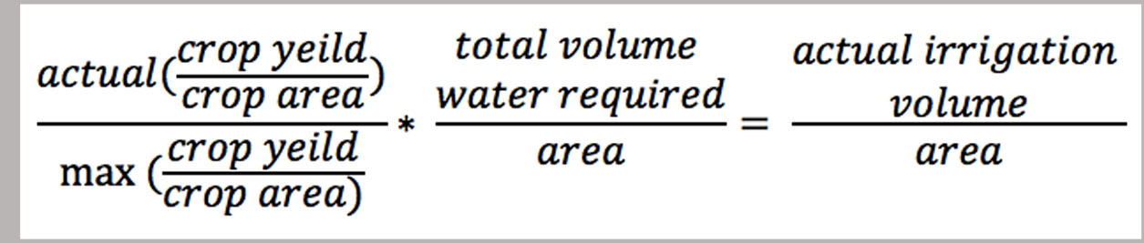
- Add crop types, area, and irrigation values to the model. Crop yields and cropped area are known for each district. Irrigation values will be estimated:

Once the model is appropriately calibrated, it will be run forward in time to provide insight on future groundwater conditions. Different pumping and agricultural scenarios will also be run to determine the effectiveness of potential remediation strategies. This research also provides a foundation for future developments in the design of accurate numerical models for understanding groundwater flow given relatively sparse data.
Sources:
Agricultural Planning Atlas of Punjab. Punjabi University, Patiala: Sardar Devindar Singh Kang.
APHRODITE’s Water Resources. (n.d.). Retrieved June 20, 2016, from http://www.chikyu.ac.jp/precip/english/ Department of Irrigation | Government of Punjab. (n.d.). Retrieved June 20, 2016, from http://irrigation.punjab.gov.in/OldVersion/statistics.html FAO – Water Development and Management Unit – Crop Water
Evaluation of Aquifer Parameters in the Riverain Tract, Punjab, India. India Hindustan Publish Corperation.
Ground Water Surveys and Investigation. New Delhi: Ashish Publishing House. Mahajan, G., & Singh, B. D. (1979).
Ground Water Year Book Punjab And Chandiharh (UT) 2014 – 2015. (2015, September). Central Ground Water Board Ministry of Water Resources, River Development and Ganga Rejuvenation Government of India. Mahajan, G. (1995).
Information: Maize. (n.d.). Retrieved June 20, 2016, from http://www.fao.org/nr/water/cropinfo_maize.html
Rao, M. B. R. (1973). The Subsurface Geology of the Indo-Gangetic Plains. Journal of the Geological Society of India, 14(3), 217 – 242.
Russo, T., Devineni, N., & Lall, U. (2015). Assessment of Agricultural Water Management in Punjab, India, Using Bayesian Methods. In Sustainability of Integrated Water Resources Management (pp. 147 – 162). Switzerland: Springer International Publishing. Singh, G. B. (1986).
Updated: April, 2017