
Introduction
The nine dimensional haystack is a model used to quantify the parameter space Earth observers must pick through to rule out the existence of signals originating from extraterrestrial civilizations. This frame work outlines the parameter space to be searched rather than putting exhaustive bounds on the existence of DExtra Terrestrial Intelligence (ETI). We have outlined the phase space of each parameter necessary to model the search with this framework. The complete haystack’s 9D phase space can be quantified with a 9D integral, so maximum and minimum bounds are required for each parameter. Specifying bounds allows us to express each search as a fraction, which ultimately allows for a more complete quantitative picture of how much of the cosmic haystack SETI observers have searched to date. Along with upper and lower bounds, we have included the relevant quanities from our recent Green Bank Observation to serve as examples of what an observer might input into this framework.
Our final product will be a calculator into which observers will put values (in correct units). This calculator will then output the fraction of the cosmic haystack that the observation spans. The intention is that this model will accommodate all useful parts of the EM spectrum by treating them as separate initially, then combining them once fractions are calculated individually. The frame work includes both radio and microwave. In the future, it should be extended to the Optical and NIR which is of special consequence due to the recent efforts in this direction (ONIRSETI) to search for laser beacons
Dimensions –
- Sensitivity –
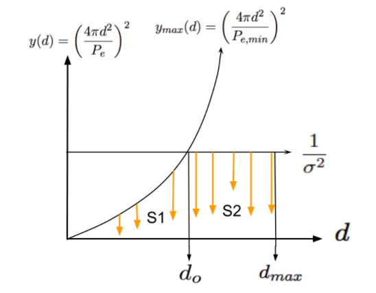
Here we aim to quantify the minimum intensity of a signal that the receiver can detect. We have defined sensitivity with units of W/m2 (not Janskys). These units were chosen because we are interested in Equivalent Isotropically Radiated Power (EIRP) at a given distance.
For example: on a plot of sensitivity vs bandwidth, the integral with our maximum and minimum as upper and lower bounds represents the volume searched in this 2D parameter space.
Axis Bounds : At each distance d the bound has been defined as a 10^13 W EIRP signal at distance d.
- Transmitter BW –
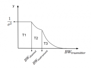
The sensitivity of detection varies with the transmitter bandwidth. Therefore this axis is meant to quantify the fraction of transmitter bandwidths that we can rule out.
The bandwidth parameter space has three distinct regions: (1) unresolved, (2) resolved and (3) resolved and greater than instrument bandwidth . For the unresolved case, the transmitter bandwidth is less than our instrument’s channel bandwidth. Second, the transmitter bandwidth is greater than our instrument’s channel bandwidth (resolved) and less than our instrument bandwidth. In the last region, the transmitter bandwidth is greater than our instrument bandwidth and hence cannot all be captured by the observer.
Axis Bounds : For the GBT observation these bounds are defined by our L-band observation.
- Distance (Space)

Instead of defining space by number of stars searched, we have opted to define space by three spatial dimensions: distance away and solid angle on the sky. The main motivation for this choice is to allow for the possibility of off-planet transmitters (i.e. intelligent civilizations could conceivably place transmitters in locations other than that of their home planet). Also, we multiply this fraction by the solid angle ratio. This is the beam width squared of the telescope Omega divided by 4pi. The total volume you have to search is the volume of the galaxy.
Axis Bounds : Maximum distance is the end of the galaxy.
4. Frequency –
The maximum bound is chosen because if you go any higher, your data will be dominated by a quantum limit . At 300GHz, it is no longer clear that the instrument of choice should be a radio telescope; it may be that a bolometer is more effective. We have chosen the minimum bound because longer wavelengths experience internal reflection by our ionosphere.
Axis Bounds: 0.01 GHz to 300 GHz
The lower bound is set by the ionospheric transmission boundary.

5. Polarization –
In the radio, the telescopes detect both polarizations. Hence, for the purposes of this framework, this axis is search complete and the fraction is 1.
Note: This fact will have to be checked for archival searches, since they might not necessarily be dual pol. If not dual pol, then polarization fraction will be 0.5 .
6. Repetition Rate –
The repetition time is the inverse of the rate at which the signal has to repeat itself for us to be able to detect it. The fraction ruled out will have the bounds defined above.
Taking a second observation (without changing any parameters) increases the number of repetition rates ruled out. A second observation can be stacked with previous observations to also increase sensitivity, but only if the observations being stacked are < a few hours apart (due to barycentric motion / doppler drift rate changing the rest frequency). Therefore a 10 minute integration will cover twice the volume as a 5 minute integration.
Axis Bounds : 0 to 100 years
7. Modulation –
Defined as the ability to identify the signal, and identify its extra terrestrial origins if detected. This would be especially pertinent when this framework is extended to the optical, and can then include the Kepler database and the TESS database to search for anomalies (like Tabby’s star).
How likely are you at catching a signal?
How wide a net must be cast to catch the signal?