Brandon Bocklund

In class, it was discussed that shifting k points off of a grid on the lattice could be used to greatly increase the effective number of k points generated by symmetry operations on the k points in the irreducible Brillouin zone (IBZ). Later when discussing the exercises of chapter 3 in Density Functional Theory: A Practical Introduction (Sholl and Steckel, John Wiley & Sons, Inc., 2009), Professor Sofo mentioned that shifting the k points should never be done in hexagonal lattices. This article will explain the idea behind Monkhorst-Pack grids used in most codes, elucidate the reasoning behind not shifting the k points grid off of the gamma point in hexagonal lattices, and give an example for the k points convergence of an hcp-Mg crystal.

k point grids and Monkhorst-Pack

Periodic crystal properties can be calculated by integrating a periodic function, \( f \), over the Brillouin zone (BZ), \( I = \int_{BZ} f(k) d^3 k \). Baldereschi [1] identified that a special point exists in the BZ that give an average value of \( f \) over the BZ, \( I = \int_{BZ} f(k) d^3 k = \frac{\left( 2\pi \right)^3}{\Omega} \bar{f} \), where \( \Omega \) is the primitive cell volume. This efficiently avoiding the computational expense of evaluating the k points over a dense grid. Each special point is unique to a Bravais lattice. A particular point, \( k^* \) in the BZ can be picked that gives an approximation of integrating over the BZ.

Chadi and Cohen [2] extended the simplification of Baldereschi to several points in the BZ and Monkhorst and-Pack [3] generalized this concept by showing that a set of k points on an evenly spaced grid on the reciprocal lattice vectors generates a plane wave expansion of \(f(k)\) in reciprocal space and that the grid maintains the symmetry of the periodic function, in this case: the symmetry of the point group of the lattice. For more details on the derivation, please refer to original work by Monkhorst and Pack [3].

The key contribution of Monkhorst and Pack’s construction of a is that calculations only need to be performed at symmetrically distinct points in the IBZ, rather than throughout the entire Brillouin zone. Practically, a user specifies the number of k points in each direction, \( N_1 \), \( N_2 \), and \( N_3 \) for a 3 dimensional lattice, and the grid is generated by \( k = u_1 b_1 + u_2 b_2 + u_3 b_3 \), where \( b_i \) are the reciprocal lattice vectors. \( u_i \) scale the reciprocal vectors by \( u_i = \frac{2x – N_i -1}{2 N_i} \) for \( x \in 1, 2, …, N_i \). Practically, these k points are calculated, the IBZ is determined, then the symmetry operations of the lattice are applied to tile the k points in the BZ. Each k point in the IBZ is assigned a weight that represents how many of the total k points can be represented by the symmetry reduced k point, \( w_{k_{i, IBZ}} = \frac{N_{k_{i, IBZ}}}{N_{k_{I, BZ}}} \), where \(N_{k_{i, IBZ}}\) and \(N_{k_{i, BZ}}\) are the number of k points in the IBZ and in the BZ, respectively, that are symmetric. The value of the function being approximated by the k point in the IBZ is calculated and multipled by the weight of that irreducible k point.

Because the Monkhorst-Pack approach approximates a function that is periodic with the same symmetry as the lattice, it is required that the generated k points have the same symmetry as the lattice. Figure 1 shows a square lattice with a 4×4 Monkhorst-Pack k points grid (a) and a 5×5 k point grid (b). A square lattice has 4-fold rotation symmetry about the origin and mirror planes on the (1, 0) and (1, 1) planes (in the center each way and along the diagonals of the square, the other planes are generated by rotation). If the k points in the IBZ are tiled through the space, the resulting k point grid in the IBZ will have the same symmetry as the lattice (in these cases, no new k points will be generated in the BZ than those represented already in Figure 1).

Figure 1. 4×4 (a) and 5×5 (b) Monkhorst-Pack k point grids on a square lattice with reciprocal lattice vectors of unit length. The irreducible Brillouin zone is highlighted in red.

Figure 2 shows the generated k points grid for the hexagonal case with a 4×4 grid in (a), 5×5 in (b) and 4×4 with a shift to the gamma point in (c). In the same sense as with the square lattice, we can imagine applying the symmetry operations to the hexagonal grid: a six-fold rotation about the origin and a mirror plane on the (1, 0) plane and the (\(\sqrt(3)\)/2, 1/2) plane (again, the other mirror planes are generated through rotations). Applying these operations to the grids in Figures 2 (a) – (c) leads to new points being generated for (a) that do not have the same symmetry as the hexagonal lattice. In (b) and (c), where the grids are both centered on the gamma point, the symmetrized k points retain the same symmetry as the lattice. This is the reason for required gamma centered grids for hexagonal lattices.

Figure 2. 4×4 (a), 5×5 (b), and 4×4 shifted (c) Monkhorst-Pack k point grids on a hexagonal lattice with reciprocal lattice vectors of unit length. The irreducible Brillouin zone is highlighted in red.

It should be noted that hexagonal lattices are only a special (but common) case to consider. In fact, all k point grids must retain the same symmetry as the underlying lattice, so for Bravais lattices care must be taken that any k point grid not centered on the gamma point (either by an unshifted even grid or a shifted odd grid) does not lose the symmetry of the underlying lattice. Some codes, such as VASP, check for this and warn the user or refuse to run.

Example of shifted grids for hexagonal lattices

In this section we compare the effects of different grids on the total energy of hcp-Mg. For brevity, the details of energy cutoff convergence and choice of lattice parameters for Mg will not be discussed. For details on how to do this for hcp materials, see the other posts. The plane wave density functional theory calculations are performed using the VASP (version 5.4.4) [4] using the PBE exchange-correlation functional [5] and PAW psueodpotentials [6] The linear tetrahedron method [7] is used for numerical integration of the BZ. An energy cutoff of 280 eV was chosen and the SCF loop was converged to an energy difference of \( 10^{-6} \) eV.

In Figure 3, the relative energies of the k points grid is plotted with respect to the number of k point divisions. In VASP, k point grids with the Monkhorst-Pack scheme can be generated two different ways:

1. An unshifted Monkhorst-Pack grid (line 3 starts with “M” in the KPOINTS file)
2. A Monkhorst-Pack grid that is always shifted to be centered on the gamma point (line 3 starts with “G” in the KPOINTS file). The shift will always result in one k point being on the gamma point.

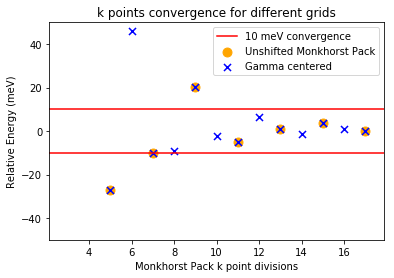
Figure 3. Relative energy of hcp Mg with respect to the number of Monkhorst-Pack divisions for unshifted Monkhorst-Pack grids and grids that are always shifted to the gamma point. In red are the limits for 10 meV convergence.

Note that VASP will not perform the calculation for k point grids that don’t retain the same symmetry, so only grids with odd divisions are plotted for the unshifted Monkhorst-Pack scheme. It can be seen that the energies exactly co-incide for the gamma centered grids and Monkhorst-Pack grids with odd divisions, suggesting that the KPOINTS used might be the same. VASP outputs a file called IBZKPT when it runs that gives the k points used and their weights in the same format as the KPOINTS file. Using the IBZKPT file, we can confirm that the same k points are used in the IBZ for the unshifted Monkhorst-Pack scheme and the gamma centered Monkhorst-Pack scheme (as we would expect, given Figure 2). The beginning of this file with the k points fractional coordinates in reciprocal space and the calculated weights are given below.

Automatically generated mesh
 6
Reciprocal lattice
 0.00000000000000 0.00000000000000 0.00000000000000 1
 0.33333333333333 0.00000000000000 0.00000000000000 6
 0.33333333333333 0.33333333333333 0.00000000000000 2
 0.00000000000000 0.00000000000000 0.33333333333333 2
 0.33333333333333 0.00000000000000 0.33333333333333 12
 0.33333333333333 0.33333333333333 0.33333333333333 4

References

[1] Baldereschi, Mean-Value Point in the Brillouin Zone. Phys. Rev. B 7, 5212–5215 (1973)
[2] Chadi & Cohen, Special Points in the Brillouin Zone. Phys. Rev. B 8, 5747–5753 (1973)
[3] Monkhorst & Pack, Special points for Brillouin-zone integrations. Phys. Rev. B 13, 5188–5192 (1976)
[4] G. Kresse, J. Furthmüller, Efficient iterative schemes for ab initio total-energy calculations using a plane-wave basis set, Phys. Rev. B. 54 11169–11186 (1996)
[5] Perdew, Burke, Ernzerhof, Generalized Gradient Approximation Made Simple, Phys. Rev. Lett. 77 (1996)
[6] P.E. Blöchl, Projector augmented-wave method, Phys. Rev. B. 50 (1994)
[7] Blöchl, Jepsen, and Andersen, Phys. Rev. B 49, 16 223 (1994)

Appendix

Code to generate the lattices

This Python code can be run in a Jupyter Notebook. It requires that ASE, matplotlib, and numpy are installed.

%matplotlib inline
import matplotlib.pyplot as plt
import numpy as np
from ase.dft.kpoints import monkhorst_pack

# Square lattice, Figure 1
# user input
kpt_mesh = [np.array([4, 4, 1]), np.array([5, 5, 1])]
lattice_name = "Square"
b1 = np.array([1, 0])
b2 = np.array([0, 1])
IBZ_path = ([0, 0.5, 0.5], [0, 0.5, 0])
plt_min_max = (-0.5, 1.1)
figname = "Fig1.png"

fig, axes = plt.subplots(1,len(kpt_mesh), figsize=(4*len(kpt_mesh), 4))

for mesh, ax in zip(kpt_mesh, axes):
    # run
    twod_pts = monkhorst_pack(mesh)[:, :2]
    orig = np.array([0, 0])

    d = twod_pts[:,:1]*b1 + twod_pts[:,1:2]*b2
    x = d[:,0]
    y = d[:,1]

    ax.scatter(x, y)
    ax.plot([0, b1[0]], [0, b1[1]], label=r'$b_1$')
    ax.plot([0, b2[0]], [0, b2[1]], label=r'$b_2$')
    ax.plot(IBZ_path[0], IBZ_path[1], label='IBZ', c='red')
    ax.set_title("{} lattice, {}x{} MP mesh".format(lattice_name, mesh[0], mesh[1]))
    ax.set_xlim(*plt_min_max)
    ax.set_ylim(*plt_min_max)
    ax.legend()
    if figname is not None:
        fig.savefig(figname)

# Hexagonal lattice, Figure 2
# user input
kpt_mesh = [np.array([4, 4, 1]), np.array([5, 5, 1]), np.array([4, 4, 1])]
shifts = [np.zeros(2), np.zeros(2), np.array([0.1875, np.sqrt(3)*0.0625])]
lattice_name = "Hexagonal"
b1 = np.array([1, 0])
b2 = np.array([0.5, np.sqrt(3)/2])
IBZ_path = ([0, np.sqrt(3)/4, np.sqrt(3)/4], [0, 0.25, 0])
plt_min_max = (-0.7, 1.1)
figname = "Fig2.png"


fig, axes = plt.subplots(1,len(kpt_mesh), figsize=(4*len(kpt_mesh), 4))

for mesh, shift, ax in zip(kpt_mesh, shifts, axes):
    # run
    twod_pts = monkhorst_pack(mesh)[:, :2]
    orig = np.array([0, 0])

    d = twod_pts[:,:1]*b1 + twod_pts[:,1:2]*b2 + np.tile(shift, (twod_pts.shape[0], 1))
    x = d[:,0]
    y = d[:,1]

    ax.scatter(x, y)
    ax.plot([0, b1[0]], [0, b1[1]], label=r'$b_1$')
    ax.plot([0, b2[0]], [0, b2[1]], label=r'$b_2$')
    ax.plot(IBZ_path[0], IBZ_path[1], label='IBZ', c='red')
    if not np.all(np.isclose(shift, 0)):
        ax.set_title("{} lattice, {}x{} MP mesh\n({:0.5f}, {:0.5f}) shift".format(lattice_name, mesh[0], mesh[1], shift[0], shift[1]))
    else:
        ax.set_title("{} lattice, {}x{} MP mesh\nNo shift".format(lattice_name, mesh[0], mesh[1]))
    ax.legend()
    ax.set_xlim(*plt_min_max)
    ax.set_ylim(*plt_min_max)
    if figname is not None:
        fig.savefig(figname)