Category Archives: H on Cu(111)

Convergence exploration for k points and cutoff energy based on the model of a hydrogen atom on Cu(111) surface HCP site

Introduction

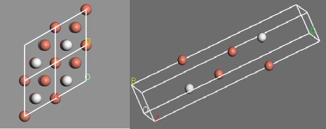
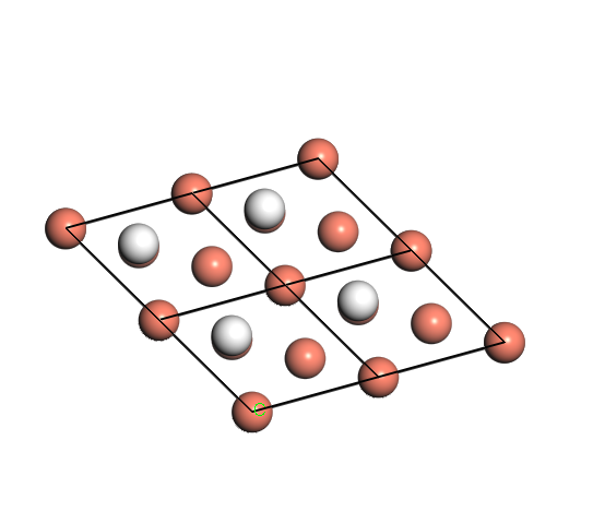
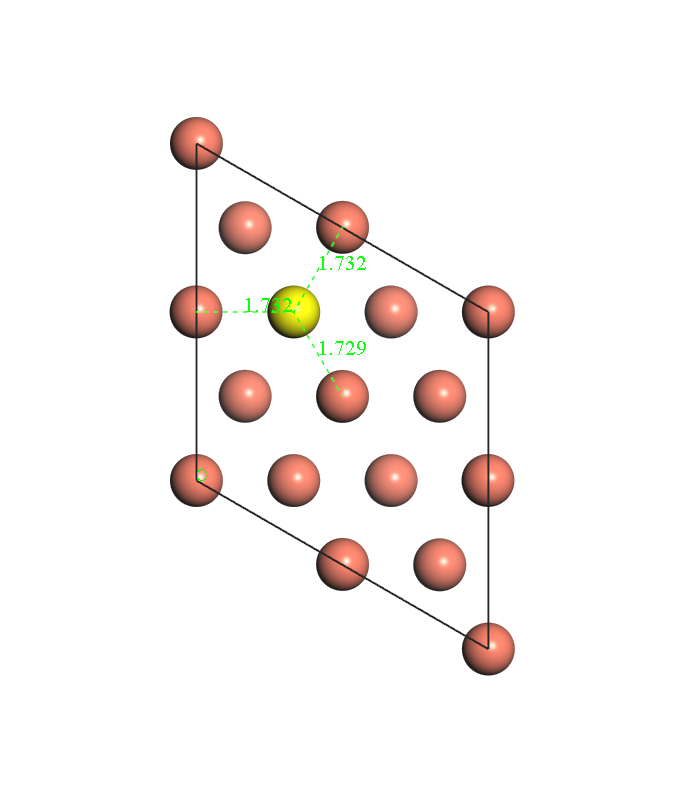
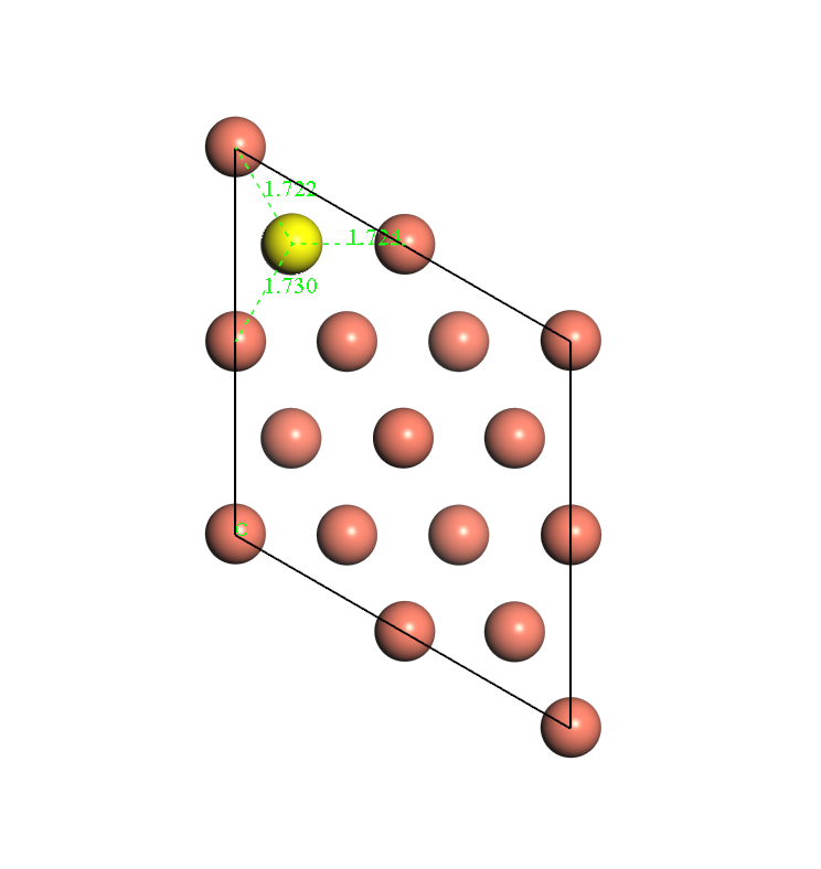
This post is aimed at exploring the convergence of k points and cutoff energy. The model chosen here is one hydrogen atom on copper(111) surface HCP site.  The model of copper surface in one periodic volume is 1*1 unit cell in x-y plane and 4 layers in z direction. Vacuum is in z direction and its thickness is 10 Å.

Fig. 1 A top view of the model

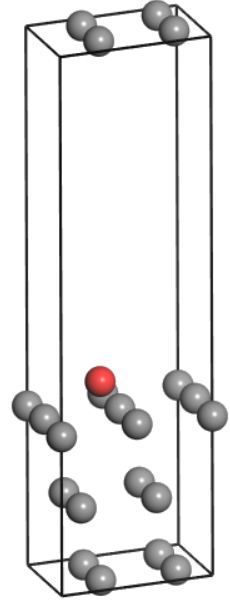
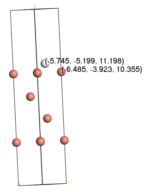
Fig. 2 A side view of the model


CASTEP tool package is adopted for all calculations in this post [1].

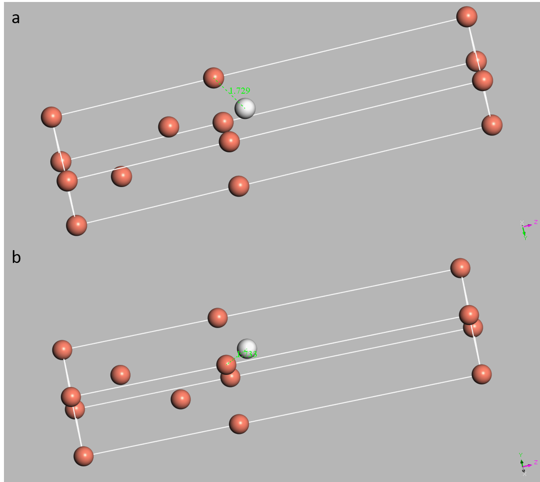
For the purpose of simplifying the model and reducing computational cost, during geometry optimization,  all copper atoms and x, y coordinates of H are fixed and H is just allowed to move in z direction.

The initial calculation setting for geometry optimization is:

Functional: GGA PBE [2]

Pseudopotentials: OTFG ultrasoft

Relativistic treatment: Koelling-Hamon

SCF tolerance: 5*10^-7 eV/atom

Max SCF cycles: 100

Dipole correction: not applied

Cutoff energy: 600 eV

K points: 11*11*2

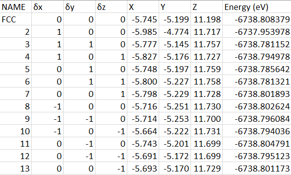
After geometry optimization, a series of finite difference calculations are conducted by only changing cutoff energy and k points. The movement step  adopted here is 0.05Å in z direction, up and down respective to equilibrium position. The energy difference of three positions is adopted as convergence indicator, named as ΔE.

Since the only freedom here is H movement in z direction, we define the indicator ΔE to be:

\begin{equation} \Delta E =  E(+ \delta z) + E (- \delta z) – 2 E_0 \end{equation}

E0 is the energy for the system at equilibrium. E(+δz) means the energy of the system after H moving away from the copper surface in z direction with one step (0.05Å). E(-δz) has the opposite meaning.

The indicator is the numerator of mass-weighted Hessian Matrix and since the denominator is constant for this model the indicator shows the convergence of vibration frequency of H actually.

Results

Cutoff energy

K mesh is fixed at 11*11*2, and just cutoff energy is changed.

Calculation results are shown in Table 1. and Fig. 1. All energies are in the unite of eV.

E_cut 1/E_cut E0 E(+δz) E(-δz) ΔE
300 0.003333333 -6734.207987 -6734.201406 -6734.203442 0.011127427
350 0.002857143 -6737.770064 -6737.765333 -6737.763871 0.010923297
400 0.0025 -6738.585562 -6738.581103 -6738.578878 0.011143039
450 0.002222222 -6738.741297 -6738.736179 -6738.735176 0.011238688
500 0.002 -6738.76858 -6738.763114 -6738.7628 0.011244911
550 0.001818182 -6738.777772 -6738.772113 -6738.772165 0.011265619
600 0.001666667 -6738.78372 -6738.777944 -6738.778252 0.011242922
700 0.001428571 -6738.789645 -6738.783725 -6738.784317 0.011249237

Table 1

Fig. 3 the plot of ΔE vs reciprocal of cutoff energy

So A numerical guess rather than a strictly theoretical conclusion based on these data points is when we have an infinitely large cutoff energy for a fixed geometry with some specific setting, we should converge to a certain number for our indicator ΔE. When the cutoff energy goes smaller, we will have more numerical noise and the numbers will potentially deviate away from the ‘true value’ which is given by the infinitely large cutoff energy. The guess is visualized in Fig. 2.

Fig. 4 a schematic plot showing the extreme situation of cutoff energy’s effect on ΔE

A part of Fig. 2 that is zoomed up to show details is shown in Fig. 3.

Fig.5 a detailed part of Fig. 2

As we can see from Fig. 3, a smaller cutoff energy will potentially give a larger deviation from the ‘true value’. Or smaller cutoff energies will give a larger range of deviation from the ‘true value’.

The exact pattern may be dependent on the indicator of convergence we choose. The practical implementation of cutoff energy in CASTEP codes will affect the pattern as well. But the tendency could be general for cutoff energy’s convergence path.

And for this specific model, the difference of ΔE from 600eV to 700eV is around 0.000006 eV. If our tolerance for ΔE is at the magnitude of 0.00001 eV, choosing 600eV as our cutoff energy under the condition of using 11*11*2 for k points is acceptable. And the converged ΔE could be 0.01124 eV.

K points

Cutoff energy is fixed at 600 eV, and just k points is changed.

First, a test for k points in z direction is conducted. The results are shown in Table 2. All energies are in the unit of eV. The difference of energies calculated from k*k*2 and k*k*1 is at the magnitude of 10^-5 eV. k means the number of k points in x or y direction. If we raise our tolerance for energy difference up to 0.0001, it could be acceptable to use ‘1’ for z direction and just change the number of k points in x and y direction for following calculations in order to reduce the computational cost.

k mesh E0 k mesh E0 energy difference between k*k*2 and k*k*1
7x7x1 -6738.709562 7x7x2 -6738.709586 -2.4000E-05
8x8x1 -6738.731698 8x8x2 -6738.73171 -1.2075E-05
9x9x1 -6738.75047 9x9x2 -6738.750535 -6.4864E-05
10x10x1 -6738.769096 10x10x2 -6738.769144 -4.8546E-05
11x11x1 -6738.783685 11x11x2 -6738.78372 -3.5046E-05
12x12x1 -6738.775101 12x12x2 -6738.775133 -3.2509E-05
13x13x1 -6738.800963 13x13x2 -6738.800992 -2.8743E-05
14x14x1 -6738.774423 14x14x2 -6738.774454 -3.1116E-05
15x15x1 -6738.795033 15x15x2 -6738.795057 -2.4665E-05

Table 2a

In order to make the convergence test for k points in z direction more convincing, we calculate 7*7*3 as well.

k mesh 7*7*1 7*7*2 7*7*3
E0 -6738.709562 -6738.709586 -6738.709615
Energy difference from 7*7*1 0 2.4E-05 5.3E-05

Table 2b

As we can see, the energy difference between 7*7*3 and 7*7*1 is still at 10^-5 magnitude.

Results for a series of k*k*1 calculations are shown in Table 3 and Fig. 4. Energies are in the unit of eV.

k-mesh k 1/k E0 E(+δz) E(-δz) ΔE
3*3*1 3 0.333333333 -6739.47838 -6739.489468 -6739.45571 0.011580839
5*5*1 5 0.2 -6738.742468 -6738.746554 -6738.727462 0.010920861
7x7x1 7 0.142857143 -6738.709562 -6738.706263 -6738.702423 0.010438667
9x9x1 9 0.111111111 -6738.75047 -6738.743514 -6738.746635 0.010791582
11x11x1 11 0.090909091 -6738.783685 -6738.777909 -6738.778218 0.01124229
13x13x1 13 0.076923077 -6738.800963 -6738.796022 -6738.79491 0.010994729
15x15x1 15 0.066666667 -6738.795033 -6738.791071 -6738.788042 0.010951909
16x16x1 16 0.0625 -6738.770667 -6738.766317 -6738.763964 0.011054494

Table 3

Fig. 6 the plot of ΔE vs 1/k

Based on data points in Fig. 4, we can see the convergence of k points has a similar pattern with cutoff energy. Difference of ΔE from 15*15*1 to 16*16*1 is still at the magnitude of 10^-3 eV, which is not desirable. We can do the fitting to get the converged number of ΔE, the ‘true value’, given by infinitely large k points. The candidate fitting function could be a*exp(bx)*sin(c*x) and a,b,c are parameters needing to be fitted. Since the number of data points here is small the fitting would be loose. Instead of calculating more data points, another cheap way of approximating the ‘true value’ is doing average for last five ΔE numbers (9*9*1, 11*11*1, 13*13*1, 15*15*1, 16*16*1). The average is 0.0110070008 eV and if we truncate it to 10^-4 eV, we have 0.0110 eV, which is different from above-mentioned number, ‘0.01124 eV’, calculated from the setting of 11*11*2 as k points and 600 eV as cutoff energy. The inconsistency of using k*k*2 and k*k*1 in different tests could result in some difference. But as mentioned before, the difference should be minor. The main reason might be the average is adopted here. The number of converged ΔE could be 0.011 eV with the cost of losing some precision.

Conclusion

Based on the ΔE = 0.011 eV, vibration frequency of H on Cu(111) surface HCP site in z direction is 3.266*10^13 Hz.

Regardless of particularity of codes and models, we can say that the energy difference ΔE defined above calculated from DFT methods by using a specific k points and cutoff energy can only be trusted in a range around that number given by the infinitely large k points and cutoff energy. The larger the k points and cutoff energy is, the narrower the range is.

Acknowledge

The optimized geometry for all calculations in this post is provided by Mark Hagemann. Mark Hagemann and Brett Green also did calculations for E0 in Table 1; calculations in Table 2; calculations for E0 in Table 3 from 7*7*1 to 16*16*1.

The energy numbers for 7*7*1, 7*7*2 shared by Mark were ‘final energy(E)’ but other energy numbers are ‘final free energy(E-TS)’. So I changed Mark’s data for E0 at 7*7*1, -6738.689838(E), to -6738.709562(E-TS) for consistency.

Thank Mark and Brett for sharing their data.

Reference

  1. First principles methods using CASTEP” Zeitschrift fuer Kristallographie 220(5-6) pp. 567-570 (2005) S. J. Clark, M. D. Segall, C. J. Pickard, P. J. Hasnip, M. J. Probert, K. Refson, M. C. Payne
  2. J. P. Perdew, K. Burke, and M. Ernzerhof Phys. Rev. Lett. 77, 3865 (1996)


Impact of the Zero Point Energy Correction to Hydrogen Adsorption Sites on the Cu (111) Surface

Purpose of Calculation

In this post, we calculate the zero point energy (ZPE) correction to an adsorbate atom on a surface. The ZPE contributes to the energy of the system, and can affect which binding site on a surface corresponds to the minimum energy arrangement. The ZPE arises from the fact that the adsorbed atom is free to oscillate while still bound to the surface, behaving as a quantum mechanical oscillator. One of the most important features of such an oscillator is, of course, that its lowest energy mode is not a zero energy mode, but a finite energy mode. So, when calculating a system with an adsorbate, we this finite energy (the ZPE) becomes a correction to our calculation. Since the correction energy is the energy of a harmonic oscillator, we expect that the energy should be largely determined by our spring constant (the “stiffness” of our bond” and the mass of the bonded atom. Therefore, the ZPE correction should be most important to atoms such as hydrogen. To demonstrate this, we calculate the ZPE correction for Hydrogen adsorbed at two sites on the Cu (111) surface: the hcp site and the fcc site.

Figure 1: A supercell (2×2) of Hydrogen (red) adsorbed on the (111) surface of copper

Theory of the Zero Point Energy

The ZPE for a quantum mechanical oscillator is given by the sum of the frequencies of the vibrational modes of the system, multiplied by constants. These vibrational modes can be obtained from the eigenvalues of the mass-weighted Hessian matrix of the system. The Hessian matrix is composed of double partial derivatives of the system energy with respect to the displacement of atoms in the system. The energy we calculate for each atomic displacement is in eV, and energy in general relates to time through energy equals mass times distance squared, divided by time squared. The Hessian matrix removes the distance dependence of the Hessian elements. If we then divide out the mass dependence, the elements are in units of inverse seconds squared. If we then take the square root of the eigenvalues of this system, the resulting quantity will be in units of inverse time, as our frequencies should be. In our system, since we are assuming the copper surface’s movement during vibrations will be negligible compared to the hydrogen atom’s movement, the hydrogen atom should be displaced along the x, y, and z direction with an appropriate step size to calculate the second derivatives of energies with respect the movements.

Numerically, we calculate the derivatives using the finite difference approximation. The diagonal elements can be calculated using the first equation below, and the off-diagonal elements can be calculated using the second.[3]

\begin{equation} H_{ii} \cong \frac{E(\delta x_{i})+E(-\delta x_{i})-2E_{0}}{\delta x_{i}^2} \end{equation}
\begin{equation} H_{ij} \cong \frac{E(\delta x_{i}, \delta x_{j})+E(-\delta x_{i},-\delta x_{j})-E(\delta x_{i}, -\delta x_{j})-E(-\delta x_{i}, \delta x_{j})}{4\delta x_{i}\delta x_{j}} \end{equation}


Delta x represents the displacement of the hydrogen atom along direction i or j, and E-naught is the energy when hydrogen is not displaced.

Now, we can diagonalize the Hessian matrix, obtaining the eigenvalues, from which we can directly calculate the vibrational frequencies, using [3]:

\begin{equation} \nu_{i} = \frac{\sqrt{\lambda_{i}}}{2\pi} \end{equation}

where lambda represents the indexed eigenvalue, and nu is the corresponding frequency. These eigenvalues are of the mass-weighted Hessian matrix, which can be obtained be dividing the Hessian matrix by the square root of the mass of the atoms that are being displaced. In our case, this means we should divide by the square root of the mass of hydrogen. Each frequency then contributes an energy

\begin{equation} E_{ZPE} = \frac{h\nu_{i}}{2} \end{equation}

to the ZPE, where h is Planck’s constant.

Calculation Methodology

The ZPE correction to hydrogen on the copper (111) surface is calculated at two sites. For these calculations, we cleave the (111) surface from bulk copper, and then form a super 2×2 supercell, so that both sites are present with all nearest neighbors for interactions. We include three layers of Cu atoms. The lattice parameters are 5.11 angstroms, 5.11 angstroms, 14.17 angstroms (a, b, c). The calculation cell contains 12 unique copper atoms and one unique hydrogen atom. We perform the calculations using Dmol3, which uses a localized basis set [1]. All calculations are performed with the Perdew-Burke-Ernzerhof (PBE) [2] exchange-correlation functional, a Generalized Gradient Approximation (GGA) functional.The on-the-fly basis set is calculated by generating a radial function calculated by solving the density equations on the fly at three hundred points on a logarithmic radial mesh for each atom. This radial function is then multiplied by appropriate spherical harmonics for each atom. We use the DNP basis set method for this calculation. All electrons are included in the Dmol3 calculations. Our SCF threshold is 10^-6 Ha.

We select a 4x4x2 k-point mesh, which test calculations show to be converged to within 0.025 Ha. The cutoff for the localized basis set is set to 4.9 angstroms, and ten angstroms of vacuum space is included in the supercell. We select 0.05 angstroms as our displacement distance. This displacement is selected after calculating the diagonal elements for the Hessian matrix for displacements of 0.01, 0.05 and 0.1 angstroms. 0.01 angstrom displacements did not provide significant changes in the calculated energy relative to the level to which energy was converged. At 0.05 angstroms, there is a significant change in calculated energy, so we elect to use 0.05 angstroms, so that our displacement does not become so large that the finite difference approximation of the derivative is no longer a good approximation.

Results

Calculations were performed for both the hcp and fcc sites with 0.05 angstroms of displacement in each possible combination of directions. Results are shown Table 1.

Displacements (Angstroms)Energy (Ha)
XYZhcpfcc
000-19685.479636-19685.485998
-0.0500-19685.478748-19685.485904
0.0500-19685.480315-19685.485877
0-0.050-19685.480315-19685.485869
00.050-19685.478748-19685.485911
00-0.05-19685.479381-19685.485882
000.05-19685.479387-19685.485759
-0.05-0.050-19685.478283-19685.485797
-0.050-0.05-19685.478244-19685.485762
0-0.05-0.05-19685.479899-19685.485717
-0.050.050-19685.4791136-19685.485798
-0.0500.05-19685.47871-19685.485685
0-0.050.05-19685.477772-19685.485658
0.05-0.050-19685.479407-19685.485774
0.050-0.05-19685.480249-19685.485728
00.05-0.05-19685.479387-19685.485771
0.050.050-19685.479321-19685.485763
0.0500.05-19685.479899-19685.485665
00.050.05-19685.477165-19685.485691

From these values, we can then calculate the appropriate Hessian matrices for each site. As a visual example, the hcp Hessian is

\begin{bmatrix} 8.36\times10^{18} & 9.166\times10^{18} & 8.16\times10^{18} \\ 9.166\times10^{18} & 8.36\times10^{18} & 9.5\times10^{17} \\ 8.16\times10^{18} & 9.5\times10^{17} & 2.016\times10^{19}\end{bmatrix}

Here, all the elements are in units of the square root of mass multiplied by inverse seconds square. Dividing all the elements by square root of the mass of hydrogen and diagonalizing, we obtain the eigenvalues: 5.1258×10^31, 3.1687×10^32 and 6.361×10^32 for the hcp site. For the fcc site, the eigenvalues are 2.0753×10^32, 2.1371×10^32 and 3.4746×10^32. The total ZPE correction for each of these eigenvalues is 0.607 eV for the hcp site and 0.576 eV for the fcc site.

These ZPE corrections are significantly large. Our convergence for the energy calculation, 0.0025 Ha corresponds to approximately 0.068 eV. The corrections are almost an order of magnitude larger than our energy convergence, meaning they represent a correction that should absolutely be included in our calculation. Also of note are that the hcp and fcc corrections differ but hundredths of an eV. When we minimized the energies for each location of the hydrogen atom before displacement, the hcp position was lower than the fcc site by approximately 0.15 eV. As a result, this correction does not change the preferred site from hcp to fcc, but it is still a significant contribution, and illustrates how the ZPE correction can be vital to the proper treatment of systems. With a more stringent convergence of the energy in the calculation, we would be able to better resolve the exact ZPE correction, but at this time, the computational resources were not sufficient to do so in a time-efficient manner.

In addition, possible other sources of error include contributions from copper atoms that Dmol3’s localized basis set do not properly capture, isolation of the hydrogen atom and other similar concerns. In an actual adsorption reaction, there will not be a single hydrogen atom with no other nearby hydrogen on the surface. Instead, something like half the sites might be occupied, or some other, more complex situation. This calculation does not reflect such concerns.

References

[1]  Delley, J., Fast Calculation of Electrostatics in Crystals and Large Molecules; Phys. Chem. 100, 6107 (1996)

[2]  John P. Perdew, Kieron Burke, and Matthias Ernzerhof, “Generalized Gradient Approximation Made Simple”, Phys. Rev. Lett. 77, 3865 – Published 28 October 1996; Erratum Phys. Rev. Lett. 78, 1396 (1997)

[3] D. Sholl and J. Steckel, Density Functional Theory: A Practical Introduction. (Wiley 2009)

Hydrogen atoms adsorbed on Cu(111) surface

In this project, the absorption of H atom in the Cu (111) surface is analyzed and calculated. The H atom absorbed on Cu(111) can bind in two distinct threefold sites, the fcc sites and hcp sites shown in Figure 1. The energy difference between these two sites are calculated using Castep and the vibrational frequencies of H in each site is analyzed by calculating the elements of the Hessian matrix using finite-difference approximations. Then based on the vibrational frequencies, the zero-point energy can be obtained.

Figure 1. The absorption of H atom in the Cu (111) surface. the grey atoms are the H atoms and the red atoms are the Cu atoms. The H atoms are in the hcp sites (a) and fcc sites (b).

1. The slab model

As shown in Figure 1, an asymmetric slab model of 4 layers are used for the calculation. During the calculation, the two bottommost layers are fixed at bulk positions and all remaining atoms allowed to relax at z direction to obtain the optimized structures.

2. The optimized structures

For both two sites, the geometry optimization in the Castep is used to obtain the optimized structures, which are shown in Figure 2. We can also get the energy difference between these two structures. for hcp structure, the energy is -6738.743eV. For fcc structure, the energy is -6738.755eV. So the energy difference is 0.012eV. And since the energy of hcp structure is larger than the fcc structure, the fcc structure is more stable than the hcp structure.

Figure 2. The optimized structures for H atoms at the hcp sites (a) and fcc sites (b). The distances are 1.729 Ångstrom in a and 1.733 Ångstrom in b.

The calculation parameters for geometry optimization are listed here:
Atomic and pseudo atomic structure for H: 1s1
Atomic structure for Cu: 1s2 2s2 2p6 3s2 3p6 3d10 4s1
pseudo atomic structure for Cu: 3d10 4s1
Functional: GGA PBE
Cut off energy: 408.2eV
k-point set: 9*9*1
Energy convergence tolerance: 1.0e-005eV/atom
Force convergence tolerance: 0.03eV/Å
Stress convergence tolerance: 0.05GPa
Displacement convergence tolerance: 0.001Å

3. The vibrational frequencies

To obtain the vibrational frequencies, we need to get the Hessian matrix first. Using finite-difference approximations, the elements in the Hessian matrix can be obtained by the equation:

Table 1 shows the calculated energy and the Hessian matrix. Then the frequencies can be obtained by the equation:

λi is the eigenvalue of Hessian matrix. So we can get the frequencies shown in Table 2. The vibrational frequencies can be seen from the wave numbers of the vibrations. All the energy shown in these two table have 3  significant digits after the decimal place because we can already see the energy differences. All the Hessian matrix are shown in SI.

Table 1 The calculated energy and the Hessian matrix for hcp structure (a) and fcc structure (b).

Table 2 The eigenvalues of Hessian matrix, the vibrational frequencies and the zero-point energy for hcp structure (a) and fcc structure (b).

4. The zero-point energy correction

Since we have get the vibrational frequencies, the zero-point energy can be calculated by the equation E=∑(hv)/2.So as shown in Table 2, the total zero-point energy for hcp structure is 0.185eV and the total zero-point energy for fcc structure is 0.192eV. Then after considering the zero-point energy, the energy difference between fcc and hcp structures is 0.0046eV.

5. Conclusion and Discussion

In this project, the absorption of H atoms binding in two distinct threefold sites, the fcc sites and hcp sites on Cu (111) surface is calculated. Without considering the zero-point energy, the energy difference for these two structures is 0.012eV. With considering the zero-point energy, the energy difference for these two structures is 0.0046eV.

In this project, I assume that the H vibrations were uncoupled from the metal atoms in the surface and calculate the vibrational frequencies only moving the H atom. But this assumption is too simple and the vibrations should be more complicated in a real system. For example, we can consider the coupling between H atom and neighboring Cu atoms, which would be an interesting project for the future.

6. Reference

[1] S. J. Clark, M. D. Segall, C. J. Pickard, P. J. Hasnip, M. J. Probert, K. Refson, M. C. Payne, “First principles methods using CASTEP”, Zeitschrift fuer Kristallographie 220(5-6) pp. 567-570 (2005)

Energy differences between hydrogen atoms absorbed on the Cu (111) fcc and hcp sites with(out) zero point energy included

1. Project Description

This project aims to calculate the vibrational frequencies and zero point energy (ZPE) of one hydrogen absorbed on face centered cubic (fcc) site and hexagonal close packed (hcp) site of Cu (111) surface. Energy calculation was performed using density functional theory (DFT) with CASTEP[1]. Exchange -correlation was treated in the generalized gradient approximation (GGA), as parameterized by Perdew, Burke, and Ernzerhof (PBE) [2]. The following valence electron configurations were employed in the potentials: 1s1 for H, and 3d10 4s1 for Cu.  Psedupotentials were used in place of other electrons, with core radii of 1.996Å  for Cu, and 0.599Å for H. The Brillouin zone integration was performed using a 9*9*1 Monkhorst-Pack k-point grid, and energy cutoff is 450eV. The SCF tolerance is 2.0e-6 eV/atom, and self-consistent dipole correction along the Z-axis is applied to the asymmetric slab.

2. Geometry optimization and energy calculation of two initial configurations

We will calculate the energies of hydrogen atoms adsorbed on two different threefold sites, the face centered cubic (fcc) site and hexagonal close packed (hcp) site, on Cu (111) surface. For each initial fcc and hcp configuration, we built four layers of Cu atom in the 10 Å slab and place one H atom near the surface (Figure 1&2).  Then we would optimize geometry with bottom three layers of Cu fixed, and both first layers of Cu and hydrogen moved freely. After geometry optimization of the structure,  the energy is calculated with the most stable relative Cu and hydrogen positions.

Figure 1. Top-down view of hydrogen atoms absorbed on FCC (Left) and HCP (Right) site of Cu (111) surface

Figure 2. Side view of hydrogen atoms absorbed on FCC (Left) and HCP (Right) site of Cu (111) surface after surface relaxation

3. Hessian Matrix

We aim to calculate the Hessian Matrix by deriving energies of various configurations with slight hydrogen displacement. Sholl and Steckel (2009) suggest a good finite-difference displacements range from 0.03-0.1Å [3]. In this project, we use finite-difference with 0.06 Å along x, y, and z direction, and energies will be calculated in 12 different configurations. The minimum energy for HCP and FCC configurations are -6738.805279 eV and -6738.808379 eV; and the atom position with minimum energy is marked with δx=δy=δz=0 (Table 1).

Table 1. Energies of displacements in HCP (Upper) and FCC (Lower) configurations, with a finite-difference of 0.06 Å

The Hassian matrix is calculated by second derivative of energies with displacement [3], for diagonal element, the Hessian matrix is calculated by:

\begin{equation} H_{ii}=(\frac{\partial^2 E}{\partial x_{i}^2}) \simeq \frac{E(x+\delta x_{i})+E(x-\delta x_{i})-2E_{0}(x)}{\delta x_{i}^2} \end{equation}

For off-diagonal element, the Hessian matrix is calculated by:

\begin{equation} H_{xy}=(\frac{\partial^2 E}{\partial x \partial y}) \simeq \frac{E(x+\delta x, y+\delta y)+E(x-\delta x, y-\delta y)-E(x-\delta x, y+\delta y)-E(x+\delta x, y-\delta y)}{4\delta x\delta y} \end{equation}

Thus the Hessian matrix for HCP and FCC configurations are:

4. Vibrational frequencies and zero point energy (ZPE) calculation

We can calculate the vibrational frequencies and zero point energy from the mass-weighted Hessian Matrix A, where the elements in the matrix A are [3]:

\begin{equation} A_{ij} = H_{ij} / m_i \end{equation}

The eigenvectors e and eigenvalues λ of matrix A satisfy Ae = λe. And vibrational frequencies νare obtained from the eigenvalues λi of the matrix product A[3],

\begin{equation} \nu_i = \sqrt{\lambda}/2\pi \end{equation}

Thus the eigenvalues and vibrational frequencies of the HCP and FCC mass-weighted Hessian matrix are (Table 2):

Table 2. The calculated eigenvalue and frequencies in HCP and FCC configurations

and zero point energy (ZPE) is obtained by [3]:

\begin{equation} E_{ZPE} = \Sigma_i \frac{ h \nu_i}{2} \end{equation}

Thus the zero point energy of HCP and FCC configurations are 0.175347eV and 0.623748eV.

5. Conclusion

The energies are summarized in Table 3. The energy differences between HCP and FCC configurations without ZPE are 0.003100eV, with ZPE are -0.445301eV. That’s to say, Without including ZPE, hydrogen on the FCC site has a lower energy than HCP sites (0.003100eV), which means hydrogen in FCC site is more stable. With ZPE included, hydrogen on the FCC site has a higher energy than HCP (0.445301eV), which means HCP site is more forved. Therefore, light atoms, such as hydrogen, should consider the influence of the zero point energy.

Table 3. A summary of energy with(out) ZPC when hydrogen absorbed on HCP and FCC sites.


Reference

[1]. S. J. Clark, M. D. Segall, C. J. Pickard, P. J. Hasnip, M. J. Probert, K. Refson, M. C. Payne, “First principles methods using CASTEP”, Zeitschrift fuer Kristallographie 220(5-6) pp. 567-570 (2005)

[2]. J. P. Perdew, K. Burke and M. Ernzerhof, “Generalized gradient approximation made simple”. Phys. Rev. Lett. 77, 3865 (1996).

[3]. Sholl, D. S., & Steckel, J. A. (2009). What is density functional theory? (pp. 1-33). John Wiley & Sons, Inc.


Energy and frequency calculation for hydrogen on Cu(111)

Introduction

Hydrogen atoms on Cu(111) can bind in two distinct threefold sites, HCP and FCC. This post is aimed at showing energy difference between these two sites without and with zero point energy correction by using DFT calculation.

For harmonic oscillator, in classical mechanics, the energy for equilibrium state is zero kinetic energy plus potential energy E0; But in quantum mechanics, due to Heisenburg uncertainty principle, the energy changes to: \begin{equation} E = E_0 + \Sigma_i \frac{h \nu_i}{2} \end{equation}

E0 is still the potential energy and ν is the vibrational frequency of the oscillator. Zero point energy is defined as: \begin{equation} E_{ZPE} = \Sigma_i \frac{ h \nu_i}{2} \end{equation}

Normally, zero point energy is not trivial for light atoms, like H.
In order to get zero point energy, vibration frequencies of H on Cu surface are needed and these frequencies are calculated from mass-weighed Hessian Matrix A, which has a relation with Hessian matrix H:
\begin{equation} A_{ij} = H_{ij} / m_i \end{equation}
where mi is mass of the atom associated with ith coordinate. In this post m =1.00794*1.66054*10^-27 kg. The eigenvalues of matrix A λ could give vibration frequencies by: \begin{equation} \nu_i = \sqrt{\lambda}/2\pi \end{equation}

Constructing Hessian Matrix requires us to do second-order differentiation for energy to coordinate: \begin{equation} H_{ij} = (\frac{\partial E}{\partial x_i \partial x_j})_{x=0} \end{equation}

which could be obtained from finite difference approximation. The method used in this post is the simple one which involving three points in one differentiation:

\begin{equation} H_{ij} \simeq \frac{E(\delta x_i, \delta x_j) – 2 E_0 + E(- \delta x_i, – \delta x_j)}{\delta x_i \delta x_j} \end{equation}

The model built in this post is H on the Cu(111) surface with three layers, vacuum above the surface is 10 Å. 2*2 supercell is adopted in case the hydrogen atoms in periodic structure are too close.

Before individual energy calculations, geometry optimization is conducted first. The hydrogen atom is put near the HCP site (or FCC site). Bottom two layers are fixed and the first layer and hydrogen are allowed to relax. After geometry optimization is finished, the distance between H atom and nearest three Cu atom could be checked. Fig. 1, 2 and 3 show the diagrams of the model. Fig. 1 shows that after geometry optimization, the distances between H atom and nearest three Cu atoms are close. So does Fig. 2. Fig.3 shows the side-view of the model.


Fig. 1 diagram for HCP site after geometry optimization

Fig. 2 diagram for FCC site after geometry optimization


Fig. 3 side-view of ‘H on Cu(111)’ model


Based on the geometry optimized, H atom is moved to three directions (x, y, z) according to elements in Hessian Matrix and energy calculation is conducted after each movement. The move step is 0.04Å.

Functional: GGA PBE[1]; k points: 5*5*1 ; cutoff energy: 408.2 eV; SCF tolerence: 2.0*10^-6 eV/atom; Pseudopotentials: OTFG ultrasoft, for Cu: inner shell is 1s2 2s2 2p6 3s2 3p6, outer shell is 3d10 4s1, for H: outer shell is 1s1; dipole correction is included since the model is not symmetric.

(‘CASTEP’ calculation module[2] is adopted for all calculations)

Calculation results

HCP site

Table 1 shows the calculation results at HCP site. δx means movement of H atom in x direction. δy and δz have similar meaning. δx=δy=δz=0 means the result of geometry optimization. ‘1’ means one movement which is 0.04Å.

Table 1.

δx δy δz Energy (eV)
0 0 0  -2.01835196E+004
1 0 0  -2.01834837E+004
1 1 0  -2.01834811E+004
1 0 1  -2.01835046E+004
0 1 0  -2.01834837E+004
1 1 0  -2.01834811E+004
0 1 1  -2.01835050E+004
0 0 1  -2.01835070E+004
1 0 1  -2.01835046E+004
0 1 1  -2.01835050E+004
-1 0 0  -2.01834834E+004
-1 -1 0  -2.01834815E+004
-1 0 -1  -2.01834479E+004
0 -1 0  -2.01834837E+004
-1 -1 0  -2.01834815E+004
0 -1 -1  -2.01834479E+004
0 0 -1  -2.01834499E+004
-1 0 -1  -2.01834479E+004
0 -1 -1  -2.01834479E+004

Mass-weighted Hessian matrix calculated based on data in Table 1:

[  4.31362677e+29          2.29142726e+29             2.59356062e+29]

[  2.29142726e+29          4.29567826e+29             2.58159494e+29]

[  2.59356062e+29          2.58159494e+29             4.92387633e+29]

Eigenvalues of the matrix are 9.51368753 e+29, 2.01335272 e+29, 2.00614111 e+29.

Vibration frequencies of H atom at HCP site (s^-1) are 1.5524*10^14, 0.7141*10^14, 0.7129*10^14.

Zero point energy for H at HCP site is 0.6161 eV.


FCC site

Table 2 shows the calculation results at FCC site.

Table 2.

δx δy δz Energy (eV)
0 0 0  -2.01835358E+004
1 0 0  -2.01834780E+004
1 1 0  -2.01834759E+004
1 0 1  -2.01835094E+004
0 1 0  -2.01834777E+004
1 1 0  -2.01834759E+004
0 1 1  -2.01835091E+004
0 0 1  -2.01835112E+004
1 0 1  -2.01835094E+004
0 1 1  -2.01835091E+004
-1 0 0  -2.01834783E+004
-1 -1 0  -2.01834765E+004
-1 0 -1  -2.01834259E+004
0 -1 0  -2.01834784E+004
-1 -1 0  -2.01834765E+004
0 -1 -1  -2.01834261E+004
0 0 -1  -2.01834280E+004
-1 0 -1  -2.01834259E+004
0 -1 -1  -2.01834261E+004

Mass-weighted Hessian matrix calculated based on data in Table 2:

[  6.89821314e+29          3.56577192e+29             4.07730464e+29]

[  3.56577192e+29          6.91017881e+29             4.08029606e+29]

[  4.07730464e+29          4.08029606e+29             7.92127857e+29]

Eigenvalues of the matrix are 1.51030097 e+30, 3.33850851 e+29, 3.28815230 e+29.

Vibration frequencies of H atom at FCC site (s^-1) are 1.9559*10^14, 0.9196*10^14, 0.9126*10^14

Zero point energy for H at FCC site is 0.7833 eV.

Conclusion:

Table 3 shows the energies of H at two three-hold sites on Cu(111) without and with zero point energy.

Table 3

Energy (eV) HCP FCC E(HCP) – E(FCC)
Without ZPE -20183.5196 -20183.5358 0.0162
With ZPE -20182.9034 -20182.7525 -0.1509

When zero point energy is not included, the H atom on FCC site has lower energy. But when zero point energy is included, the H atom on HCP site has lower energy. Zero point energy is important for light atoms, like H and should be considered for systems involving light atoms.

Reference:

  1. J. P. Perdew, K. Burke, and M. Ernzerhof Phys. Rev. Lett. 77, 3865 (1996)
  2. First principles methods using CASTEP” Zeitschrift fuer Kristallographie 220(5-6) pp. 567-570 (2005) S. J. Clark, M. D. Segall, C. J. Pickard, P. J. Hasnip, M. J. Probert, K. Refson, M. C. Payne
  3. R. Ryberg, Carbon-Monoxide Adsorbed on Cu(100) Studied by Infrared-Spectroscopy, Surf. Sci. 114 (1982), 627 641.

Vibrations of Hydrogen on a Copper(1 1 1 ) Surface

In this project a hydrogen atom will be adsorbed to a Cu(1 1 1) surface and the vibration modes of the hydrogen atom will be calculated.  There are two sites where the hydrogen atom can be stably adsorbed, the fcc site and hcp site, as such both sites will be considered. 

For these calculations the functional PBE was use, along with OTFG ultrasoft pseudopotentials, the Koelling-Hamon relativistic treatment, a k-point grid of 11x11x1 and a energy cutoff of 600eV. The dipole correction was not used for these calculations as the corrections were smaller that the level of precision guaranteed by the k-point grid and energy cut selection.

Pseudo atomic configuration Cu: 3d10 4s1

Pseudo atomic configuration H: 1s1

Optimization

To calculate this first the hydrogen atom was place on either the hcp or fcc lattice site of a Cu(111) surface and then the geometry of the system was optimized holding the bottom three layers fixed and allowing the top layer of the Cu surface and the hydrogen atom move freely. For the convergence, the energy convergence was set to 10-5 eV/atom, the max force was set to 0.03 eV/A, the max stress was set to 0.05 GPa, and the max displacement was set to 0.001A. The results of the optimization can be seen in Figures 1 and 2.

Figure 1: Optimized structure for hydrogen adsorbed to fcc site.

Figure 2: Optimized structure for hydrogen adsorbed to hcp site.

Construction of the Hessian Matrix

In this work, only the vibrations of the hydrogen are wanted, so an approximation that can be used is to only allow the hydrogen atom to move while constructing the Hessian. This will simplify the Hessian to a 3×3 matrix. From the following equation the Hessian matrix can be calculated.

H_{ij} = \bigg(\frac{\partial^2 E}{\partial x_i \partial x_j}\bigg) 
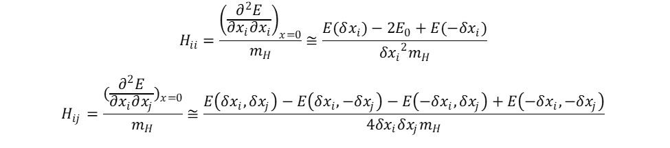
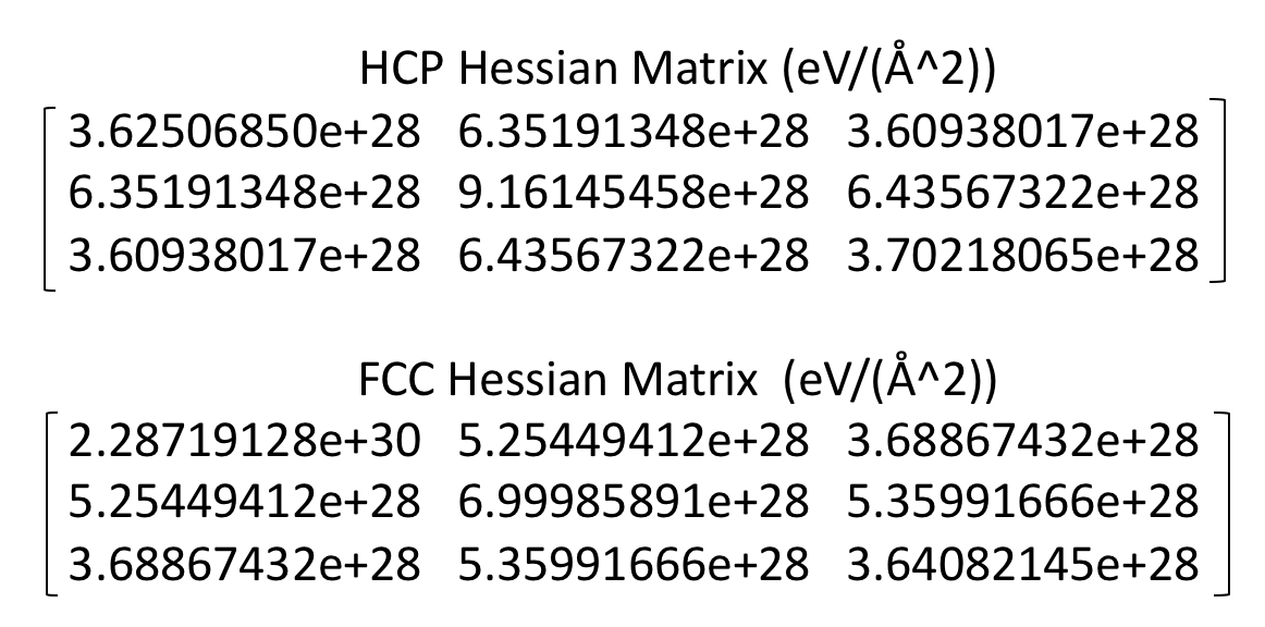
= \frac{E(\delta x_i, \delta x_j) - 2E(x_0)+ E(-\delta x_i, -\delta x_j)}{\delta x_i \delta x_j}

Using a displacement of 0.1A the Hessian matrix was computed and then divided by the mass of a hydrogen atom to get the mass-weighted Hessian matrix whose matrix elements are given by the following,

A_{ij} = H_{ij}/m_i

Then the eigenvalues and eigenvectors of the mass-weighted Hessian, A,  were calculated using the following relation.

\vec{A}\vec{e} = \lambda \vec{e}

Once the eigenvalues, \lambda_i, where found the normal mode frequencies, \nu_i, were calculated using the following relation.

\nu_i = \frac{\sqrt{\lambda_i}}{2\pi}

The results of these calculations for the hydrogen at the fcc site and hcp site are given in Tables 1 and 2 respectively.

Table 1: Normal mode frequency and Eigenvector for H atom is fcc site.
Eigenvectors()
Normal ModeFrequency (cm-1)xyz
1742.7-0.1880.769-0.611
2375.90.787-0.254-0.562
3366.7-0.588-0.586-0.558

Table 2: Normal mode frequency and Eigenvector for H atom is hcp site.

Eigenvectors()
Normal ModeFrequency (cm-1)xyz
1740.9-0.182 -0.763-0.620
2372.7 0.7880.264-0.557
3363.2-0.5890.590-0.553

Zero-point Energy Correction

The zero point energy for a quantum mechanical system is not that of the classical system, the corrected form is as the following,

E = E_0 +\sum_i \frac{h \nu_i}{2}

This correction is 0.0921eV for the the system with the hydrogen at the fcc site and 0.0915eV for the system with the hydrogen at the hcp site.

Conclusion

The difference in the energy of the hydrogen adsorbing to the fcc site and the hydrogen adsorbing to the hcp site is 0.0154eV. Taking into account the zero-point energy correction the difference shrinks to 0.0149eV

Zero point energy of H on Cu(111) hollow sites


This project aims to find zero point vibrational energy (ZPVE) for H atom adsorbed at Cu(111) hollow site through calculating Hessian matrix, which was built through second order finite difference approximation.

H adsorption optimization
The geometry optimization was performed in Material Studio with CASTEP Calculation Package [1]. The functional of Perdew Burke, and Ernzerhoff was employed [2]. Cu bulk was first optimized with medium SCF tolerance. Energy cutoff of 480 eV and 9 X 9 X 9 K points sampling were used. The pseudopotential was solved through Koelling-Harmon treatment. After Cu optimization, 111 surface was cut from bulk and H atom was place at hollow hcp site. K points of 11 X 11 X 1 was applied for slab optimization. Figure 1 shows optimized configuration, in which four layers of Cu was chosen and 20 angstrom vacuum was built above the surface to ensure no interaction between super cells.


Figure 1. Optimized H adsorption at Cu (111) hollow hcp site


Figure 2. Optimized H adsorption at Cu (111) hollow fcc site

Energy of structure with 0.05 angstrom H displacement at hcp site

deltaxdeltaydeltazE(eV)
0
00-5057.904815339
-0.0500-5057.900058684
0.0500-5057.900254389
0-0.050-5057.899918579
00.050-5057.900491436
00-0.05
-5057.902027622
000.05-5057.897504906
0.050.050-5057.895183611
0.05
-0.05
0-5057.894736028
-0.050.050-5057.896567514
-0.05-0.050-5057.895964697
0.0500.05-5057.893632073
0.050-0.05-5057.896676147
-0.0500.05-5057.893493162
-0.050-0.05-5057.896416514
00.050.05-5057.893875845
00.05-0.05-5057.896914666
0-0.050.05-5057.893352868
0-0.05-0.05-5057.896277175

Energy of structure with 0.05 angstrom H displacement at fcc site

deltaxdeltaydeltazE(eV)
000-5057.908254387
-0.0500-5057.903846876
0.0500-5057.902812323
0-0.050-5057.905355245
00.050-5057.901336034
00-0.05-5057.903434736
000.05-5057.900649874
0.050.050-5057.896923968
0.05-0.050-5057.900397672
-0.050.050-5057.895898678
-0.05-0.050-5057.900587944
0.0500.05-5057.896058663
0.050-0.05-5057.897022898
-0.0500.05-5057.896937081
-0.050-0.05-5057.898270256
00.050.05-5057.894816130
00.05-0.05-5057.895334570
0-0.050.05-5057.898164719
0-0.05-0.05-5057.900003390

Then finite difference approximation was used to calculate Hessian matrix elements. The diagonal element can be obtained as equation (1) and off-diagonal element can be obtained from equation (2).
\begin{equation} H_{ii} \cong \frac{E(\delta x_{i})+E(-\delta x_{i})-2E_{0}}{\delta x_{i}^2} \end{equation}
\begin{equation} H_{ij} \cong \frac{E(\delta x_{i}, \delta x_{j})+E(-\delta x_{i},-\delta x_{j})-E(\delta x_{i}, -\delta x_{j})-E(-\delta x_{i}, \delta x_{j})}{4\delta x_{i}\delta x_{j}} \end{equation}

After calculating eigenvalues of Hessian matrix, we can calculate vibrational frequency and corresponding zero point energies, which is shown in following table.

siteZero point energy (eV)
hcp0.1893
fcc0.2001

Conclusions
In this project, we applied harmonic approximation and use finite difference approximation to calculate vibrational frequency of H atom adsorbed at the Cu(111) hollow sites and further zero point energy. According to our calculation, the zero point energy of H on hcp site is 0.1893 eV and H on fcc site is 0.2001 eV. The difference of the zero point energies between H on fcc site and hcp site are less 0.011 eV.

Reference
[1] “First principle methods using CASTEP” Zeitschrift fuer Kristallographie 220(5-6) pp. 567-570 (2005)
[2] Perdew, J. P; Burke, K; Ernzerhof, M. Phys. Rev. Lett. 1996, 77, 3865-3868

Zero Point Energy Correction of H adsorbed on Cu(111)


1. Problem Description

In this project, the zero point energy (ZPE) correction of one hydrogen atom adsorbed at two different hollow sites of Cu(111) was studied.

In order to get the zero point energy, we firstly initiated the geometry optimization to find the optimal conformation of H adsorbed on Cu(111) as a stating point, by putting the H atom at the fcc-hollow site and hcp-hollow site above the surface for about 2.0 Å. Then, to get the weighted Hessian matrix required to calculate the vibrational frequencies, the H atom was displaced with a step size of 0.05 Å or 0.10 Å along the x, y, and z direction and the corresponding energies were calculated. Different displacements were tested to confirm the correct ZPE. The weighted Hessian matrix consists of the second order derivatives of energies with respect to the displacement along different directions, multiplying the weighted factor. After that, the vibrational frequencies could be found by diagonalizing the Hessian matrix and thus, the ZPE was calculated to correct the binding energy of H at different sites.


2. Computational Method

The surface was cleaved from bulk Cu using Materials Studio along the <111> direction with three layers included. In order to minimize the interactions between periodic images of H atoms, we chose to construct a (2×2) supercell including 10 Å of vacuum space as shown in Figure 1. H atom was initially located at two different hollows site above the surface. During the geometry optimization, the upmost layer along with the H atoms were allowed to move while the bottom two layers were totally fixed at the bulk position. After the geometry optimization, the single point calculations were performed to calculate the energy with different displacement of the H atom.


Figure 1. Top-down view and side view of the Cu(111)-2×2 supercell


All the calculations were carried out using CASTEP with Materials Studio and the GGA-PBE was chosen to be the exchange-correlation functional. The pseudopotential was solved with the Koelling-Harmon atomic solver and the valence electrons were 3d10 4s1 and 1s1 for Cu and H, respectively. The energy cutoff of 408.2 eV and the k-point sampling of 6x6x2 were used. The energy cutoff and k-point sampling were tested to give a convergence within 0.02 eV. The results of convergence tests are summarized below in Table 1. The convergence criteria for force and energy were 0.02 eV/ Å and 10e-6 eV, respectively. The self-consistent dipole correction along the Z-axis was also introduced to better describe the adsorption of the H atom.

Energy Cutoff (eV) 400 408.2 410 420
Energy (eV) -20182.9745 -20183.1051 -20183.1281 -20183.1374
K-point 5x5x2 6x6x2 7x7x2 8x8x2
Energy (eV) -20183.0103 -20183.1051 -20183.0376 -20183.1224
Vacuum Space (Å) 10 11 12 13
Energy (eV) -20167.1164 -20167.1163 -20167.1157 -20167.1148

Table 1: Summary of convergence tests


3. ZPE at FCC-Hollow Site

As the only atom displaced is H in our system, there weighted Hessian matrix can be easily achieved by multiplying a factor to the Hessian matrix. In order to construct the Hessian matrix for vibrational frequency, the H atom should be displaced along the x, y, and z direction with an appropriate step size to calculate the second derivatives of energies with respect the movements.

For the diagonal elements in the Hessian matrix, the second derivative was calculated using three points as shown below in equation 1, while for the off-diagonal elements, it was calculated using four points as in equation 2.

\begin{equation} H_{ii} \cong \frac{E(\delta x_{i})+E(-\delta x_{i})-2E_{0}}{\delta x_{i}^2} \end{equation}
\begin{equation} H_{ij} \cong \frac{E(\delta x_{i}, \delta x_{j})+E(-\delta x_{i},-\delta x_{j})-E(\delta x_{i}, -\delta x_{j})-E(-\delta x_{i}, \delta x_{j})}{4\delta x_{i}\delta x_{j}} \end{equation}


Here,  dxi represents the displacement in the i direction (can be along x, y, and z direction) and  E0 is the minima energy.

In this project, the step size of 0.05 Å and 0.10 Å were both applied in order to ensure that the displacements were appropriately chosen. Due to the symmetry, there were in total 18 sets of energies of different displacements required and the results for H atom at fcc-hollow site with different step sizes are summarized below in Table 2.

Displacement Direction Energy (eV)
X Y Z Step size = 0.05 Å Step size = 0.10 Å
0 0 0 -20183.1051 -20183.1051
1 0 0 -20183.1017 -20183.0910
-1 0 0 -20183.1022 -20183.0943
1 1 0 -20183.0991 -20183.0829
-1 -1 0 -20183.0986 -20183.0773
1 -1 0 -20183.0995 -20183.0841
-1 1 0 -20183.0987 -20183.0779
1 0 1 -20183.0970 -20183.0760
-1 0 -1 -20183.0970 -20183.0704
1 0 -1 -20183.0962 -20183.0647
-1 0 1 -20183.0972 -20183.0777
0 1 0 -20183.1020 -20183.0929
0 -1 0 -20183.1022 -20183.0933
0 1 1 -20183.0970 -20183.0767
0 -1 -1 -20183.0967 -20183.0678
0 1 -1 -20183.0967 -20183.0857
0 -1 1 -20183.0974 -20183.0684
0 0 1 -20183.0996 -20183.0848
0 0 -1 -20183.1004 -20183.0776

Table 2: Summary of energies with different displacements


According to the equations above, we were able to calculate the elements in the Hessian matrices as well as the eigenvalues these matrices. Thus, the zero point energy can be calculated using the equation 3 and 4 as show below.

\begin{equation} \nu_{i} = \frac{\sqrt{\lambda_{i}}}{2\pi} \end{equation}
\begin{equation} E_{ZPE} = \frac{h\nu_{i}}{2} \end{equation}


Here,  vi is the vibrational frequency and  lambda is the eigenvalue of the Hessian matrix and h is the Planck’s constant.

For the displacements with step size of 0.05 Å, the weighted Hessian matrix is

\begin{bmatrix} 2.412\times10^{28} & 4.786\times10^{26} & -5.744\times10^{26} \\ 4.786\times10^{26} & 2.297\times10^{28} & 3.829\times10^{26} \\ -5.744\times10^{26} & 3.829\times10^{26} & 3.906\times10^{28}\end{bmatrix}

The eigenvalues are 3.90907327e+28, 2.42876582e+28, and 2.27843185e+28. Corresponding zero point energies are 0.130 eV, 0.102 eV, and 0.099 eV.

For the displacements with step size of 0.10 Å,  the weighted Hessian matrix is

\begin{bmatrix} 2.383\times10^{28} & 4.308\times10^{26} & -9.573\times10^{26} \\ 4.308\times10^{26} & 2.297\times10^{28} & 3.590\times10^{26} \\ -9.573\times10^{26} & 3.590\times10^{26} & 3.800\times10^{28}\end{bmatrix}

The eigenvalues are 3.80789093e+28, 2.39781505e+28, and 2.27653408e+28. Corresponding zero point energies are 0.128 eV, 0.102 eV, and 0.099 eV.

We can see that these two different choices bring us similar ZPE with differences less than 2%, which means that our choice of step size of the displacement is appropriate. To sum up, based on the results of 0.10 Å, the total ZPE for H atom at the fcc-hollow site is 0.329 eV. The corresponding eigenvectors are [-0.06640341, -0.91052413, -0.40808872], [0.02181974, -0.41021872, 0.91172611], and [0.99755425, -0.05163733, -0.04710732].


4. ZPE at HCP-Hollow Site

Similarly, we carried out the calculations by initially locating the H atom at the hcp-hollow site. Accordingly, the results for H atom at hcp-hollow site with different step sizes are summarized below in Table 3.

Displacement Direction Energy (eV)
X Y Z Step size = 0.05 Å Step size = 0.10 Å
0 0 0 -20183.0973 -20183.0973
1 0 0 -20183.0948 -20183.0874
-1 0 0 -20183.0937 -20183.0830
1 1 0 -20183.0913 -20183.0708
-1 -1 0 -20183.0912 -20183.0753
1 -1 0 -20183.0915 -20183.0718
-1 1 0 -20183.0916 -20183.0766
1 0 1 -20183.0897 -20183.0703
-1 0 -1 -20183.0881 -20183.0560
1 0 -1 -20183.0895 -20183.0631
-1 0 1 -20183.0889 -20183.0678
0 1 0 -20183.0945 -20183.0859
0 -1 0 -20183.0944 -20183.0857
0 1 1 -20183.0895 -20183.0697
0 -1 -1 -20183.0890 -20183.0607
0 1 -1 -20183.0889 -20183.0602
0 -1 1 -20183.0893 -20183.0692
0 0 1 -20183.0917 -20183.0768
0 0 -1 -20183.0925 -20183.0774

Table 3: Summary of energies with different displacements


For the displacements with step size of 0.05 Å, the weighted Hessian matrix is

\begin{bmatrix} 2.317\times10^{28} & 5.505\times10^{26} & 1.101\times10^{26} \\ 5.505\times10^{26} & 2.202\times10^{28} & -2.393\times10^{26} \\ 1.101\times10^{26} & -2.393\times10^{26} & 3.868\times10^{28}\end{bmatrix}

The eigenvalues of this Hessian matrix are 3.98502936e+28, 2.35385631e+28, and 2.16250165e+28. The corresponding zero point energies are 0.131 eV, 0.101 eV, and 0.097 eV.

For the displacements with step size of 0.10 Å, the weighted Hessian matrix is

\begin{bmatrix} 2.336\times10^{28} & 5.744\times10^{26} & 5.744\times10^{26} \\ 5.744\times10^{26} & 2.183\times10^{28} & 2.872\times10^{26} \\ 5.744\times10^{26} & 2.872\times10^{26} & 3.983\times10^{28}\end{bmatrix}

The eigenvalues of this Hessian matrix are 3.87576398e+28, 2.33336757e+28, and 2.17737216e+28. The corresponding zero point energies are 0.130 eV, 0.101 eV, and 0.097 eV. 

We can see that these two different choices bring us similar ZPE with differences less than 2%, which means that our choice of step size of the displacement is appropriate. To sum up, based on the results of 0.10 Å, the total ZPE for H atom at the fcc-hollow site is 0.328 eV. The corresponding eigenvectors are [-0.07002192, -0.91680843, 0.39314022], [0.01196003, -0.39485082, -0.9186674 ], and [-0.99747375, 0.05962489, -0.03861327].


5. Summary

The energies of Cu slab with the H atom adsorbed at different sites before and after ZPE correction are summarized below in Table 4.

Energy (eV) ZPE(eV) Energy with ZPE (eV)
FCC-Hollow -20183.1051 0.3297 -20182.7754
HCP-Hollow -20183.0973 0.3273 -20182.7701
Difference 0.0078 0.0024 0.0053

Table 4. Summary of ZPE at different sites


We can see that ZPE is significant for the H atom adsorbed on Cu(111) but the ZPE at different hollow sites are quite similar. The differences of the total energy with and without ZPE at different sites are both within 0.01 eV, which is very small and the adsorption energy of the H atom at these two sites are almost the same. However, such a small binding energy difference is within the range of convergence error, which means that we cannot decide which site is preferred.

Reference

  1. Clark, Stewart J., et al. “First principles methods using CASTEP.” Zeitschrift für Kristallographie-Crystalline Materials 220.5/6 (2005): 567-570.
  2. Perdew, J.P., K. Burke, and M. Ernzerhof, Generalized gradient approximation made simple. Physical review letters, 1996. 77(18): p. 3865.

Zero Point Energy of Hydrogen in Cu (111) Layers Near the Surface

In this project,  the zero point energy (ZPE) of a hydrogen atom in the 2nd and 3rd layers below a Cu (111) surface was found by calculating the Hessian matrix of the atom. To do this, the hydrogen atom was shifted by 0.1Å along the x, y, and z directions of the lattice and the energy was calculated at each location using CASTEP [1]. Using these energy values, a second order finite difference approximation was used to find the Hessian, which was then diagonalized to find the vibrational frequencies of the atom. These frequencies could then be used to calculate the ZPE of the defect by approximating its oscillations as that of a quantum harmonic oscilator [2].

These calculations were performed in Materials Studio using the GGA Perdew Burke Ernzerhof (PBE) functional. The calculations used an energy cutoff of 520eV for the b-layer substituted hydrogen and a k point sampling of 15x15x2, for a total of 225 points. For the c-layer, a 540eV cutoff and a 15x15x2 k point sampling were used. The pseudopotential was solved using the Koelling-Harmon atomic solver. For Cu, the solver used 1s2 2s2 2p6 3s2 3p6 as the interior electron shells and 3d10 4s1 as the valence shells. For H, the solver used 1s1 as the valence shell.

The cutoff value and k point sampling were determined by finding where the energy converged to a 0.01eV tolerance.

Construction of the Surface

To build the desired surface, we started with a pure metal Cu lattice. This lattice was then cleaved along the (111) axis with a thickness of 4 atoms, so as to contain both B and C layers, as well as two A layers. The bottom A layer was fixed and a vacuum slab with 10Å vacuum was constructed. Then, a hydrogen atom replaced the B layer hydrogen and a symmetric slab was constructed to balance out the dipole moment of the hydrogen in the plane wave calculations. The geometry of this surface was then optimized with a 450eV cutoff and a k-sampling of 11x11x1. This structure was then used to find the proper cutoff energy and k-space sampling to get a 0.01eV convergence. The cutoff for the B layer ended up being 520eV and the k-sampling was 15x15x2. 540eV was used for the C layer cutoff. Next, the structure was geometry optimized again using the proper cutoff and k-samplings.

Fig. 1. The appearance of the b-layer defective structure before geometry optimization was performed.

Fig. 2. The appearance of the c-layer defective structure after geometry optimization was performed.

Energy at Different Hydrogen Locations

Next, the hydrogen atoms were symmetrically shifted by 0.1Å along the x, y, and z directions as needed to construct the Hessian matrix of the atom. To get the energy of only one substitutional hydrogen, these energies were halved when calculating the Hessian matrix.

Table 1. The values of the energy of the structure with a hydrogen atom located in the B layer. Here, the atoms were shifted by 0.1Å and the new energy values of the structure were found. In order to keep the structures inverted, the atoms were moved in the opposite directions, with the chart labeling of the movement of one of the atoms.

Table 2. The values of the energy of the structure with a hydrogen atom located in the C layer.

Hessian Construction and Results

A finite difference approximation and the values from Table 1 and 2 were used to construct the Hessian matrices. The diagonal elements were found using the formula:

\begin{equation} E_{xx} = \frac{E(\Delta x, 0) – 2E(0,0) + E(-\Delta x, 0)}{ \Delta x^2} \end{equation}

and the off diagonal elements were found using the formula:

\begin{equation} E_{xy} = \frac{E(\Delta x, \Delta y) – E(-\Delta x,0) – E(0, -\Delta y) + E(-\Delta x, -\Delta y)}{4 \Delta x \Delta y} \end{equation}

These elements were then placed into a matrix in Wolfram Mathematica, which was used to find the eigenvalues of the matrix, which gives

\begin{equation} 2 \pi \nu _i = \omega _i = \sqrt{ \lambda _i} \end{equation}

Using these values and the QHO approximation, we can find the vibrational energies along each direction with:

\begin{equation} E_{ZPE} = \frac{ \hbar \omega _i}{2} \end{equation}

Yielding energies of 0.047eV, 0.047eV, and 0.033eV along the x, y, and z directions respectively for the B layer hydrogen. For the C layer, ZPE energies obtained were 0.089eV, 0.089eV, and 0.065eV respectively. This gives a total ZPE of 0.128eV for the B layer HCP hydrogen defect and 0.243eV for the C layer FCC defect. Because both structures have identical classical energies within the tolerance used for this study, these results suggest that hydrogen prefers the B layer HCP site over the C layer FCC site.

References

Vibrational Frequencies and Zero Point Energies of Hydrogen on the surface of Cu(111)

Introduction

In this post we calculate the vibrational frequencies and zero point energy (ZPE) of a hydrogen absorbed on the surface of Cu(111). This is done by first doing geometry optimization to find the preferred location of the hydrogen atom in the hcp or fcc interstitial site. After this, the hydrogen atom is perturbed from the energy minimum in increments of 0.05 Å in order to calculate the hessian matrix. The mass-weighted hessian matrix is then diagonalized to find the vibrational frequencies and thus the ZPE of the hydrogen atom.

Surface Construction

The surface of the Cu(111) with hydrogen adsorbents is modeled with 4 layers of Cu(111) and hydrogen atoms at the corresponding hcp interstitial sites on each side as seen in fig 1.

Fig. 1: Top view of hydrogen in the hcp interstitial site on the Cu(111) surface with periodic boundary conditions (left). Side view of the slab model with hydrogen in the hcp site (right).

The Cu(111) slab along with the hydrogen atoms is then centered within a vacuum slab that is 15 Å thick.

Details of the Calculations

All calculations were performed with the CASTEP package in materials studio with the GGA Perdew-Burke-Ernzerhof functional [1-2]. The pseudopotential was solved with the Koelling-Harmon atomic and 1s2 2s2 2p6 3s2 3p6 for the inner shells, while 3d10 4s1 were used for the outer shells.

Geometry optimization calculations used convergence tolerances of 10^-5 eV/atom, 0.03 eV/Å for the max force, 0.05 GPa for the max stress, and a max displacement of 0.001 Å. A rough calculation using an energy cutoff of 408 eV and a 6x6x1 k-point set is performed to get an idea of where the hydrogen atoms will relax to. After this, the energy cutoff and the number of k-points are increased until there is less than a 0.01 eV change in the system energy. A geometry optimization is then performed again to find the final location of the hydrogen atoms. Through this procedure we find that an energy cutoff of 480 eV and a 12x12x2 k-point set, corresponding to 144 inequivalent k-points is found to be acceptable.

We are then able to calculate energies around the minimum by slightly perturbing the hydrogen atoms from their preferred positions. Shifting a hydrogen direction in one direction on one surface corresponds to a shift in the opposite direction on the other surface in order to preserve the symmetry of the system. The results of these calculations for the hcp site are shown in table 1, and the results for the fcc site are shown in table 2.

dx (Å)dy (Å)dz (Å)Energy (eV)
000-6753.163
0.0500-6753.151
-0.0500-6753.147
00.050-6753.152
0-0.050-6753.152
000.05-6753.150
00-0.05-6753.153
0.050.050-6753.143
0.0500.05-6753.141
00.050.05-6753.142
0.05-0.050-6753.143
0.050-0.05-6753.141
00.05-0.05-6753.141
-0.050.050-6753.140
-0.0500.05-6753.142
0-0.050.05-6753.142
-0.05-0.050-6753.140
-0.050-0.05-6753.142
0-0.05-0.05-6753.141
Table 1: Calculations of the system energies for perturbations of the hydrogen atoms about their minima in the hcp interstitial site.
dx (Å)dy (Å)dz (Å)Energy (eV)
000-6753.134
0.0500-6753.124
-0.0500-6753.123
00.050-6753.124
0-0.050-6753.124
000.05-6753.123
00-0.05-6753.124
0.050.050-6753.112
0.0500.05-6753.115
00.050.05-6753.115
0.05-0.050-6753.112
0.050-0.05-6753.113
00.05-0.05-6753.112
-0.050.050-6753.115
-0.0500.05-6753.114
0-0.050.05-6753.115
-0.05-0.050-6753.114
-0.050-0.05-6753.111
0-0.05-0.05-6753.112
Table 1: Calculations of the system energies for perturbations of the hydrogen atoms about their minima in the fcc interstitial site.

Calculation of Frequencies and Zero Point Energies

The Hessian matrix, \(\frac{\partial^2 E}{\partial x_i \partial x_j}\), can be approximated using the data in table 1. We approximate the diagonal terms with

\[\frac{\partial^2 E}{\partial x_i \partial x_i} = \frac{E(x_i + \Delta x_i) – 2E(x_i) + E(x_i – \Delta x_i)}{\Delta x_i^2}\]

and the off-diagonal terms with

\[\frac{\partial^2 E}{\partial x_i \partial x_j} = \frac{E(x_i + \Delta x_i, x_j + \Delta x_j) – E(x_i + \Delta x_i, x_j – \Delta x_j) – E(x_i – \Delta x_i, x_j + \Delta x_j) + E(x_i – \Delta x_i, x_j – \Delta x_j)}{4 \Delta x_i \Delta x_j}\].

To convert to the mass-weighted Hessian, we can simply divide by the mass of the hydrogen atoms. We divide by 2 times the mass in order to account for both atoms. The frequencies are then given by \(\nu_i = \frac{\sqrt{\lambda_i}}{2 \pi}\), where \(\lambda_i\) are the eigenvalues of the mass-weighted Hessian matrix.

Through this procedure we obtain vibrational frequencies of 36.9 THz, 32.7 THz, and 33.4 THz. We can then calculate the ZPE by treating these frequencies as those corresponding to ground states of independent quantum harmonic oscillators:

\[E_{ZPE} = \sum\limits_{i} \frac{\hbar \omega_i}{2}\]

This gives a ZPE of 0.213 eV for the hydrogen in the hcp interstitial site.

For the fcc site, this same procedure gives vibrational frequencies of 32.1 THz, 31.8 THz, and 31.1 THz. These correspond to a ZPE of 0.196 eV

Conclusions

In this post, we constructed a Cu(111) surface with hydrogen adsorbed onto either the hcp or fcc interstitial sites. We then performed geometry optimization and calculated the energies of the system when the hydrogen atoms were perturbed slightly from their minima. This allowed us to calculate the mass-weighted Hessian matrix, which was then diagonalized to give the vibrational frequencies and thus the zero-point energies. Without the inclusion of zero-point energies, the system with fcc defects is higher in energy by 0.029 eV. With the inclusion of zero-point energies, this system is greater in energy by 0.012 eV.


References

1.) First principle methods using CASTEP Zeitschrift fuer Kristallographie 220(5-6) pp. 567-570 (2005).

2.) Perdew, J.P., K. Burke, and M. Ernzerhof, Generalized gradient approximation made simple.Physical review letters, 1996. 77(18): p. 3865.