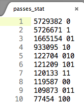
Today, I was importing table that looked like this into R:

with a command:

 r<-read.table("passes_stat",colClasses = c("integer","character"))

Why did I put an extra effort in specifying colClasses? That’s because if I wouldn’t, read.table function would have to make an educated guess about what type of the data my columns contain.

This would not only take longer (see the post here), but in this particular case it would also ruin my leading zeroes – see for example line number 5. Additionally, I might have not even noticed that it happened.

 r<-read.table("passes_stat")
 View(r)

Do you ever need to read a text file while not knowing what’s the maximum number of columns it can have? Well, I do 🙂 Turns out read.table function only looks at first five columns to determine the number of columns as ?read.table help page says:

The number of data columns is determined by looking at the first five lines of input (or the whole input if it has less than five lines), or from the length of col.names if it is specified and is longer. This could conceivably be wrong if fill orblank.lines.skip are true, so specify col.names if necessary (as in the ‘Examples’).

So what’s the workaround? Find out the maximum in advance!

  no_col <- max(count.fields(file, sep = "\t"))

  dataI <- read.table(file,sep="\t",fill=TRUE,header = F,col.names=c("chr", "start", "end", "length",1:no_col))

Since we want to fill the blanks, we will use fill=TRUE function and we may also decide to name our columns numerically as col.names does here. Thus, the columns will be named chr, start, end, length and 1, 2, 3 … maxColumn.

I found myself loading and processing huge files in R. For each  of those files, I needed to analyze many DNA motifs, so I naturally started with a for loop that, once my gargantuan file was comfortably sitting in a memory, went motif by motif and created an output for each motif separately.

This is a wonderful candidate situation for parallelization since:

• I can process each motif independently
• I can assign each motif to a single processor
• Workers/processes don’t have to communicate
• They write their output to a separate files (not a shared one so they don’t have to fight over access to it)

I quickly googled following resource by Max Gordon which demonstrates that basic implementation of parallelization (in simple cases like this one) can be very straightforward in R:

library(parallel)

list<-c("CGG","CGGT","CG","CGT") #my loooong list of motifs, shortened for illustration purposes

# Calculate the number of cores
no_cores <- detectCores() - 1
# Initiate cluster
cl <- makeCluster(no_cores,type="FORK")

print("PARALLEL")
ptm <- proc.time() #start timer
parLapply(cl, list,
 function(motif)
 processMotif(motif) #PROCESS EACH MOTIF INDIVIDUALLY
 )
stopCluster(cl)
proc.time() - ptm

print("NON-PARALLEL")
ptm <- proc.time()
for (motif in list) { 
 processMotif(motif)
}
proc.time() - ptm #stop timer

Let’s check how much time this chunk takes to run:

   user  system elapsed 

908.340 300.906 432.906

And let’s compare that with the for-loop solution:

   user  system elapsed

8544.826 3079.385 6089.453

Happy paralleLAZYing!

(The code was run on GNU/Linux with 64 processors and 500GB RAM.)