Introduction

One of the earliest posts that I made on this site described how to use Mathematica to create elevation/bathymetry profiles for the Earth, at a specified latitude. I use those profiles to have students in my 100-level non-science majors course on earthquakes and society become familiar with Earth’s surface topography and its relationship to plate tectonic features. We are now studying tsunami, and one of the activities that we complete is an estimate of the travel time from an earthquake in the eastern Atlantic to a set of cities along the east coast of the United States. The source is located near the assumed source region of the 1755 Lisbon Earthquake.

We compute the rough speed of the tsunami, \(c\) using the simple formula \(c = \sqrt{d \cdot g}\), where \(d\) is the mean depth of the water along the great-circle arc connecting the source region and the point of interest, and \(g\) is the acceleration of gravity (about \(10~m/s^2\)). In large classes I provide a map with depth of the ocean contoured and including great circle arcs connecting the source and locations of interest and students estimate the mean depth along the path. They generally do ok, but estimating the mean depth is a challenge (one worthwhile). In my smaller courses, which are taught in computer laboratories, we can do the analysis using Mathematica notebooks. Then students can plot the great circle arcs, look at the profile, estimate the mean depth, and then compute the mean depth.

The Code

Here’s the code listing to extract the elevation/bathymetry along an arc connecting points 0 and 1, specified by the latitude and longitudes (e.g. lat1,lon1)

(* city *)
lat0 = 40.66;
lon0 = -73.94;
(* eq *)
lat1 = 36;
lon1 = -10;
(* get the great-circle arc and the distance along the arc *)
gcarc = GeoPath[{{lat0, lon0}, {lat1, lon1}}, "GreatCircle"];
gcarcDistance = GeoDistance[{{lat0, lon0}, {lat1, lon1}}, UnitSystem -> "Metric"]
(**)
p0 = Framed[GeoGraphics[{Red, AbsoluteThickness[4], gcarc}, 
     GeoRange -> {{0, 70}, {-120, 20}},
     GeoProjection -> "CylindricalEquidistant", GeoZoomLevel -> 6, 
     GeoBackground -> "ReliefMap", ImageSize -> Full]];
(* extract the elevations along the great-circle arc *)
profile = GeoElevationData[gcarc, Automatic, "GeoPosition", GeoZoomLevel -> 4];
(* extract the pts = {lat,lon,elevation} from the results *)
pts = profile[[1]][[1]];
depths = #[[3]] & /@ pts;
distances =  QuantityMagnitude[GeoDistance[{pts[[1]][[1;;2]], #[[1;;2]]}, 
             UnitSystem -> "Metric"]] & /@ pts;
avg = Mean[depths];
pts = Transpose[{distances, depths}];
(* plot the elevations along the line and a dashed line for sea level *)
label =  "Mean depth along the path: " <> ToString[Round[-avg, 5]] <> " m";
(**)
p1 = ListPlot[pts, Joined -> True, 
     Frame -> {True, True, False, False}, Axes -> False, 
     Filling -> Bottom, ImageSize -> Full,
     PlotLabel -> Style[label, 18], AspectRatio -> 0.4, BaseStyle -> 14,
     Prolog -> {Blue, Dashed,
     Line[{{distances[[1]], 0}, {distances[[-1]], 0}}], Black, 
     Line[{{distances[[1]], avg}, {distances[[-1]], avg}}]}];
(**)
Column[{p0, p1}] // Print

The Output

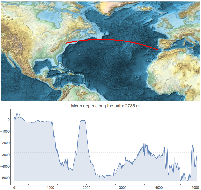
The graphics that result are show below – the dashed blue line is sea-level, the dashed black line is the mean value. A minor goal of the computation is to have students see the relationship between the mean depth and the profile.

Great circle arc between the 1755 Lisbon Earthquake epicentral region and New York City and the corresponding bathymetry profile.

The travel time for the tsunami was just over nine hours, which is not too far off from that in the Lisbon earthquake simulation from NOAA:

Students can change the latitude and longitude of the second point (the city) to estimate the travel time to other locations. To get a list of city locations, you can just ask Mathematica. I show the code as a screen shot since I used the ctrl-equals to specify the city entities. The gray-shaded region identifies the “code”, the unshaded region contains the output.

The city Saint George is how I get the location of Bermuda. Interestingly, the elevation that is displayed for Bermuda never rises above sea-level, an artifact of the sampling used to create the elevation profile.

Summary

Mathematica provides a convenient approach to extracting, processing, and plotting elevation profiles along Earth’s surface. Coupled with the ability to lookup geographic locations conveniently, the topographic profile capability can be used to allow students to compute such parameters as average tsunami speeds and arrival times.