
Purpose of Calculation
In this post, we calculate the zero point energy (ZPE) correction to an adsorbate atom on a surface. The ZPE contributes to the energy of the system, and can affect which binding site on a surface corresponds to the minimum energy arrangement. The ZPE arises from the fact that the adsorbed atom is free to oscillate while still bound to the surface, behaving as a quantum mechanical oscillator. One of the most important features of such an oscillator is, of course, that its lowest energy mode is not a zero energy mode, but a finite energy mode. So, when calculating a system with an adsorbate, we this finite energy (the ZPE) becomes a correction to our calculation. Since the correction energy is the energy of a harmonic oscillator, we expect that the energy should be largely determined by our spring constant (the “stiffness” of our bond” and the mass of the bonded atom. Therefore, the ZPE correction should be most important to atoms such as hydrogen. To demonstrate this, we calculate the ZPE correction for Hydrogen adsorbed at two sites on the Cu (111) surface: the hcp site and the fcc site.
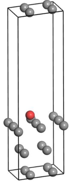
Figure 1: A supercell (2×2) of Hydrogen (red) adsorbed on the (111) surface of copper
Theory of the Zero Point Energy
The ZPE for a quantum mechanical oscillator is given by the sum of the frequencies of the vibrational modes of the system, multiplied by constants. These vibrational modes can be obtained from the eigenvalues of the mass-weighted Hessian matrix of the system. The Hessian matrix is composed of double partial derivatives of the system energy with respect to the displacement of atoms in the system. The energy we calculate for each atomic displacement is in eV, and energy in general relates to time through energy equals mass times distance squared, divided by time squared. The Hessian matrix removes the distance dependence of the Hessian elements. If we then divide out the mass dependence, the elements are in units of inverse seconds squared. If we then take the square root of the eigenvalues of this system, the resulting quantity will be in units of inverse time, as our frequencies should be. In our system, since we are assuming the copper surface’s movement during vibrations will be negligible compared to the hydrogen atom’s movement, the hydrogen atom should be displaced along the x, y, and z direction with an appropriate step size to calculate the second derivatives of energies with respect the movements.
Numerically, we calculate the derivatives using the finite difference approximation. The diagonal elements can be calculated using the first equation below, and the off-diagonal elements can be calculated using the second.[3]
\begin{equation} H_{ii} \cong \frac{E(\delta x_{i})+E(-\delta x_{i})-2E_{0}}{\delta x_{i}^2} \end{equation}
\begin{equation} H_{ij} \cong \frac{E(\delta x_{i}, \delta x_{j})+E(-\delta x_{i},-\delta x_{j})-E(\delta x_{i}, -\delta x_{j})-E(-\delta x_{i}, \delta x_{j})}{4\delta x_{i}\delta x_{j}} \end{equation}
Delta x represents the displacement of the hydrogen atom along direction i or j, and E-naught is the energy when hydrogen is not displaced.
Now, we can diagonalize the Hessian matrix, obtaining the eigenvalues, from which we can directly calculate the vibrational frequencies, using [3]:
\begin{equation} \nu_{i} = \frac{\sqrt{\lambda_{i}}}{2\pi} \end{equation}
where lambda represents the indexed eigenvalue, and nu is the corresponding frequency. These eigenvalues are of the mass-weighted Hessian matrix, which can be obtained be dividing the Hessian matrix by the square root of the mass of the atoms that are being displaced. In our case, this means we should divide by the square root of the mass of hydrogen. Each frequency then contributes an energy
\begin{equation} E_{ZPE} = \frac{h\nu_{i}}{2} \end{equation}
to the ZPE, where h is Planck’s constant.
Calculation Methodology
The ZPE correction to hydrogen on the copper (111) surface is calculated at two sites. For these calculations, we cleave the (111) surface from bulk copper, and then form a super 2×2 supercell, so that both sites are present with all nearest neighbors for interactions. We include three layers of Cu atoms. The lattice parameters are 5.11 angstroms, 5.11 angstroms, 14.17 angstroms (a, b, c). The calculation cell contains 12 unique copper atoms and one unique hydrogen atom. We perform the calculations using Dmol3, which uses a localized basis set [1]. All calculations are performed with the Perdew-Burke-Ernzerhof (PBE) [2] exchange-correlation functional, a Generalized Gradient Approximation (GGA) functional.The on-the-fly basis set is calculated by generating a radial function calculated by solving the density equations on the fly at three hundred points on a logarithmic radial mesh for each atom. This radial function is then multiplied by appropriate spherical harmonics for each atom. We use the DNP basis set method for this calculation. All electrons are included in the Dmol3 calculations. Our SCF threshold is 10^-6 Ha.
We select a 4x4x2 k-point mesh, which test calculations show to be converged to within 0.025 Ha. The cutoff for the localized basis set is set to 4.9 angstroms, and ten angstroms of vacuum space is included in the supercell. We select 0.05 angstroms as our displacement distance. This displacement is selected after calculating the diagonal elements for the Hessian matrix for displacements of 0.01, 0.05 and 0.1 angstroms. 0.01 angstrom displacements did not provide significant changes in the calculated energy relative to the level to which energy was converged. At 0.05 angstroms, there is a significant change in calculated energy, so we elect to use 0.05 angstroms, so that our displacement does not become so large that the finite difference approximation of the derivative is no longer a good approximation.
Results
Calculations were performed for both the hcp and fcc sites with 0.05 angstroms of displacement in each possible combination of directions. Results are shown Table 1.
| Displacements (Angstroms) | Energy (Ha) | |||
|---|---|---|---|---|
| X | Y | Z | hcp | fcc |
| 0 | 0 | 0 | -19685.479636 | -19685.485998 |
| -0.05 | 0 | 0 | -19685.478748 | -19685.485904 |
| 0.05 | 0 | 0 | -19685.480315 | -19685.485877 |
| 0 | -0.05 | 0 | -19685.480315 | -19685.485869 |
| 0 | 0.05 | 0 | -19685.478748 | -19685.485911 |
| 0 | 0 | -0.05 | -19685.479381 | -19685.485882 |
| 0 | 0 | 0.05 | -19685.479387 | -19685.485759 |
| -0.05 | -0.05 | 0 | -19685.478283 | -19685.485797 |
| -0.05 | 0 | -0.05 | -19685.478244 | -19685.485762 |
| 0 | -0.05 | -0.05 | -19685.479899 | -19685.485717 |
| -0.05 | 0.05 | 0 | -19685.4791136 | -19685.485798 |
| -0.05 | 0 | 0.05 | -19685.47871 | -19685.485685 |
| 0 | -0.05 | 0.05 | -19685.477772 | -19685.485658 |
| 0.05 | -0.05 | 0 | -19685.479407 | -19685.485774 |
| 0.05 | 0 | -0.05 | -19685.480249 | -19685.485728 |
| 0 | 0.05 | -0.05 | -19685.479387 | -19685.485771 |
| 0.05 | 0.05 | 0 | -19685.479321 | -19685.485763 |
| 0.05 | 0 | 0.05 | -19685.479899 | -19685.485665 |
| 0 | 0.05 | 0.05 | -19685.477165 | -19685.485691 |
From these values, we can then calculate the appropriate Hessian matrices for each site. As a visual example, the hcp Hessian is
\begin{bmatrix} 8.36\times10^{18} & 9.166\times10^{18} & 8.16\times10^{18} \\ 9.166\times10^{18} & 8.36\times10^{18} & 9.5\times10^{17} \\ 8.16\times10^{18} & 9.5\times10^{17} & 2.016\times10^{19}\end{bmatrix}
Here, all the elements are in units of the square root of mass multiplied by inverse seconds square. Dividing all the elements by square root of the mass of hydrogen and diagonalizing, we obtain the eigenvalues: 5.1258×10^31, 3.1687×10^32 and 6.361×10^32 for the hcp site. For the fcc site, the eigenvalues are 2.0753×10^32, 2.1371×10^32 and 3.4746×10^32. The total ZPE correction for each of these eigenvalues is 0.607 eV for the hcp site and 0.576 eV for the fcc site.
These ZPE corrections are significantly large. Our convergence for the energy calculation, 0.0025 Ha corresponds to approximately 0.068 eV. The corrections are almost an order of magnitude larger than our energy convergence, meaning they represent a correction that should absolutely be included in our calculation. Also of note are that the hcp and fcc corrections differ but hundredths of an eV. When we minimized the energies for each location of the hydrogen atom before displacement, the hcp position was lower than the fcc site by approximately 0.15 eV. As a result, this correction does not change the preferred site from hcp to fcc, but it is still a significant contribution, and illustrates how the ZPE correction can be vital to the proper treatment of systems. With a more stringent convergence of the energy in the calculation, we would be able to better resolve the exact ZPE correction, but at this time, the computational resources were not sufficient to do so in a time-efficient manner.
In addition, possible other sources of error include contributions from copper atoms that Dmol3’s localized basis set do not properly capture, isolation of the hydrogen atom and other similar concerns. In an actual adsorption reaction, there will not be a single hydrogen atom with no other nearby hydrogen on the surface. Instead, something like half the sites might be occupied, or some other, more complex situation. This calculation does not reflect such concerns.
References
[1] Delley, J., Fast Calculation of Electrostatics in Crystals and Large Molecules; Phys. Chem. 100, 6107 (1996)
[2] John P. Perdew, Kieron Burke, and Matthias Ernzerhof, “Generalized Gradient Approximation Made Simple”, Phys. Rev. Lett. 77, 3865 – Published 28 October 1996; Erratum Phys. Rev. Lett. 78, 1396 (1997)
[3] D. Sholl and J. Steckel, Density Functional Theory: A Practical Introduction. (Wiley 2009)
