Author: Hoang (Bolton) Tran

Problem statement [1]

Platinum (Pt) crystal structure are hypothesized to take the form of either a simple cubic (SC), a face-centered cubic (FCC) or a hexagonal closed pack (HCP) structure.

Density functional theory [2] (DFT) calculation is used to first, find the optimal lattice constant for each of the proposed structure. The optimal lattice constant is one that yields the lowest cohesive energy (E) per atom in the unit cell.  Then, the lowest cohesive energy among the three structures would indicate which structure is optimal for Pt.

Methodology

Software:

DFT calculation is carried out using CAmbridge Serial Total Energy Package (CASTEP), a plane wave basis set tool that embedded inside BIOVIA Material Studio (MS) software. [3]

Calculation:

1. DFT energy calculation setting:

• Exchange-Correlation Functional: Generalized Gradient approximations – Perdew-Burke-Ernzerhof (GGA-PBE) [4]
• Self-Consistent Field tolerance: 2E-06 eV
• Pseudo potential: On-the-fly Generated (OTFG) ultrasoft (Vanderbilt-type) [5]. Core radius: 2.4 a.u.. Core orbitals: 1s2 2s2 2p6 3s2 3p6 3d10 4s2 4p6 4d10

Cohesive energy is calculated by subtracting the atomic pseudo energy (-13042.3015 eV) from the estimated 0 K energy. All energy is in per atom basis.

2. Lattice constant optimization

Crystal structures of Pt are generated in MS with editable lattice constant.

The lattice constant for SC and FCC is a which is side length of the cubic unit cell. a is varied and the cohesive energy (E) is calculated. Data of E vs. a is then fitted to the Birch-Murnaghan (BM) equation of state [6]. Then the minimum a from the fitted function is considered as the optimal lattice constant.

The lattice constants for HCP are a and c, the basal side length and height respectively. All lattice constants are defined and optimized in its primitive cell.

3. Convergence

The energy cutoff for plane wave set is varied for a particular set of lattice constant optimization. As energy cutoff is incremented, the minimum cohesive energy is calculated until the difference with respect to result at highest energy cutoff is less than 0.01eV . This optimal energy cutoff is then used throughout all calculations.

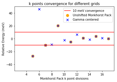
The kpoints, which represent Monkhorst-Pack sampling space [7] for the plane wave, is optimized for each crystal structure. The grid parameters for k space is varied for each set of lattice constant optimization and then optimized similarly to energy cutoff, i.e. until minimum cohesive energy does not change by more than 0.01 eV with respect to highest kpoints result.

Results

1. Energy cutoff optimization:

Simple cubic structure is chosen to be optimized in term of energy cutoff at constant kpoints of  120 (15x15x15 grid). The lattice constant a is varied from 2 to 3.5 Å and cohesive energy is extracted and fitted to BM equation. Similar procedure is then repeated for different values of energy cutoff. Figure 1 illustrate such fitting for two values of energy cutoff. Python’s scipy.optimize module [8] is used to find the minimum energy for each fitted function.

Table 1 below shows that the minimum cohesive energy goes down as energy cutoffs increases. Difference with respect to highest energy cut off (i.e. 450 eV in this case) is used as the criteria of convergence. Therefore, 400 eV point would be considered as converged because it differs from 450 eV point by less than 0.01 eV. But as to ensure good convergence throughout, 450 eV will be used as the optimal energy cutoffs for all following calculations.

Table 1. Minimum total energy at different energy cutoffs – SC

Energy cutoff (eV)	Minimum total energy (eV/atom)	Difference with respect to highest cutoff (eV)
270	-7.626	0.539
300	-8.003	0.161
350	-8.151	0.013
400	-8.164	0
450	-8.164	0

2. Simple cubic

To determine to optimal lattice constant, similar process of varying a and calculating cohesive energy and fitting it to BM equation to find the minimum point is repeated, now with different kpoints. The results are shown in table 2.

Table 2. Minimum cohesive energy at different kpoints – simple cubic

kpoints	Minimum cohesive energy (eV/atom)	Difference with respect to highest kpoints (eV)
35	-8.194	-0.040
56	-8.176	-0.022
84	-8.209	-0.055
120	-8.157	-0.003
286	-8.154	0.003

It is seen that kpoints of 120 (15x15x15 grid) is the optimal value which gives the optimal lattice constant a as 2.637 Å and minimum cohesive energy as -8.157 eV/atom

3. Face centered cubic

Kpoints convergence is again performed for FCC structure and results are shown in table 3.

Table 3. Minimum cohesive energy at different kpoints – FCC

kpoints	Minimum cohesive energy (eV/atom)	Difference with respect to highest kpoints (eV)
56	-8.659	-0.004
84	-8.643	0.012
110	-8.655	0.000
120	-8.655	0.000

The optimal kpoints as seen from the table, is 110 (10x10x10 grid) which correspond to lattice constant as 2.811 Å and minimum cohesive energy as -8.655 eV/atom.

4. Hexagonal closed pack

With two lattice constants a and c, the optimal values are found by fixing a ratio of c/a then perform similar curve fitting for minimum cohesive energy per atom.

First, ratio c/a of 1.50 is chosen to optimize in terms of kpoints.

Table 4. Minimum cohesive energy per atom at different kpoints – HCP

kpoints	Minimum cohesive energy (eV/atom)	Difference with respect to highest kpoints (eV)
3	-8.691	-0.026
14	-8.681	-0.016
36	-8.665	0
76	-8.664	0.001
136	-8.665	0

With similar interpretation as above sections, kpoints of 36 (9x9x6 grid) is optimal in performing calculation for HCP structure. This kpoints will be used for different c/a ratio.

Figure 2 illustrate the BM equation fitting for different c/a ratio. The minimum for each fitted curve is then plotted against the c/a ratio in Figure 3.

It is observed from Figure 3 that c/a ratio of 1.65 has the lowest cohesive energy/atom which is -8.674 eV/atom and lattice constants of a = 2.817 Å and c = 4.648 Å.

Conclusions

It is interesting to see that the minimum cohesive energy per atom of HCP structure is lower than that of FCC structure, which suggest that Pt prefers the HCP structure and that does not agree with what is well known [9].

It is noted, however, that the minimum cohesive energy for each configuration is found by curve fitting to the BM equation. Hence to reaffirm the result, re-calculation was done in CASTEP for each of the crystal structure, using the determined optimal kpoints and lattice constants to reevaluate this discrepancy (table 5).

Table 5. Re-calculation for energy of each crystal structure

	SC	FCC	HCP
a (A)	2.637	2.812	2.817
c (A)	-	-	4.468
Fitted minimum E (eV/atom)	-8.157	-8.655	-8.674
Re-optimized E (eV/atom)	-8.207	-8.664	-8.605

From re-calculation results, cohesive energy per atom of FCC structure is the lowest, indicating the expected result of FCC structure being the stable structure for Pt.

Retrospectively, the convergence criteria for both kpoints and energy cutoff is ±0.01 eV, therefore a meaningful comparison can only be made if difference in energy between two structures is more than 0.02 eV. The difference between fitted minimum E of HCP and FCC is 0.019 eV (third row table 5), while that of the re-calculated energy is 0.059 eV (fourth row table 5). Therefore more confidence can be given to the re-calculated results.

A method that does not require re-calculation is to fit the BM equation multiple times to converge on a good cohesive energy value. This study, instead, calculated the minimum cohesive energy after fitting the BM equation only once to roughly determine the optimal lattice constant, then re-calculate the energy at that optimal lattice constant to use for comparison between crystal structures.

Lastly, the optimal lattice constant reported in literature [9] is 3.92 Å. For this study, converting primitive to conventional FCC yields a lattice constant of 3.98 Å. The relative error is 1.5% which is a very good agreement.

Reference.

[1] Sholl, D., Steckel, J., & Sholl. (2011). Density Functional Theory (p. 46). Somerset: Wiley.

[2] R.O Jones (2015), Density functional theory: Its origins, rise to prominence, and future, Rev. Mod. Phys. 87, 897.

[3] “First principles methods using CASTEP”, Zeitschrift fuer Kristallographie 220(5-6) pp. 567-570 (2005) S. J. Clark, M. D. Segall, C. J. Pickard, P. J. Hasnip, M. J. Probert, K. Refson, M. C. Payne

[4] J. P. Perdew, K. Burke, M. Enzerhof (1996). Generalized Gradient Approximation Made Simple, Phys, Rev. Lett., 77, 3865.

[5] D. Vanderbilt (1990), Soft self-consistent pseudopotentials in a generalized eigenvalue formalism. Phys. Rev. B 41 (11), 7892-7895.

[6] Franis Birch (1947), Finite Elastic Strain of Cubic Crystals, Phys. Rev. 71, 809.

[7] H. J. Monkhorst and J. D. Pack (1976), Special points for Brillouin-zone integrations, Phys. Rev. B 13, 5188.

[8] Jones E, Oliphant E, Peterson P, et al. SciPy: Open Source Scientific Tools for Python, 2001.

[9] Hermann, K. (2011). Crystallography and surface structure (Appendix E: Parameter Tables of Crystals). Wiley‐VCH Verlag GmbH & Co. KGaA.

Brandon Bocklund

In class, it was discussed that shifting k points off of a grid on the lattice could be used to greatly increase the effective number of k points generated by symmetry operations on the k points in the irreducible Brillouin zone (IBZ). Later when discussing the exercises of chapter 3 in Density Functional Theory: A Practical Introduction (Sholl and Steckel, John Wiley & Sons, Inc., 2009), Professor Sofo mentioned that shifting the k points should never be done in hexagonal lattices. This article will explain the idea behind Monkhorst-Pack grids used in most codes, elucidate the reasoning behind not shifting the k points grid off of the gamma point in hexagonal lattices, and give an example for the k points convergence of an hcp-Mg crystal.

k point grids and Monkhorst-Pack

Periodic crystal properties can be calculated by integrating a periodic function, \( f \), over the Brillouin zone (BZ), \( I = \int_{BZ} f(k) d^3 k \). Baldereschi [1] identified that a special point exists in the BZ that give an average value of \( f \) over the BZ, \( I = \int_{BZ} f(k) d^3 k = \frac{\left( 2\pi \right)^3}{\Omega} \bar{f} \), where \( \Omega \) is the primitive cell volume. This efficiently avoiding the computational expense of evaluating the k points over a dense grid. Each special point is unique to a Bravais lattice. A particular point, \( k^* \) in the BZ can be picked that gives an approximation of integrating over the BZ.

Chadi and Cohen [2] extended the simplification of Baldereschi to several points in the BZ and Monkhorst and-Pack [3] generalized this concept by showing that a set of k points on an evenly spaced grid on the reciprocal lattice vectors generates a plane wave expansion of \(f(k)\) in reciprocal space and that the grid maintains the symmetry of the periodic function, in this case: the symmetry of the point group of the lattice. For more details on the derivation, please refer to original work by Monkhorst and Pack [3].

The key contribution of Monkhorst and Pack’s construction of a is that calculations only need to be performed at symmetrically distinct points in the IBZ, rather than throughout the entire Brillouin zone. Practically, a user specifies the number of k points in each direction, \( N_1 \), \( N_2 \), and \( N_3 \) for a 3 dimensional lattice, and the grid is generated by \( k = u_1 b_1 + u_2 b_2 + u_3 b_3 \), where \( b_i \) are the reciprocal lattice vectors. \( u_i \) scale the reciprocal vectors by \( u_i = \frac{2x – N_i -1}{2 N_i} \) for \( x \in 1, 2, …, N_i \). Practically, these k points are calculated, the IBZ is determined, then the symmetry operations of the lattice are applied to tile the k points in the BZ. Each k point in the IBZ is assigned a weight that represents how many of the total k points can be represented by the symmetry reduced k point, \( w_{k_{i, IBZ}} = \frac{N_{k_{i, IBZ}}}{N_{k_{I, BZ}}} \), where \(N_{k_{i, IBZ}}\) and \(N_{k_{i, BZ}}\) are the number of k points in the IBZ and in the BZ, respectively, that are symmetric. The value of the function being approximated by the k point in the IBZ is calculated and multipled by the weight of that irreducible k point.

Because the Monkhorst-Pack approach approximates a function that is periodic with the same symmetry as the lattice, it is required that the generated k points have the same symmetry as the lattice. Figure 1 shows a square lattice with a 4×4 Monkhorst-Pack k points grid (a) and a 5×5 k point grid (b). A square lattice has 4-fold rotation symmetry about the origin and mirror planes on the (1, 0) and (1, 1) planes (in the center each way and along the diagonals of the square, the other planes are generated by rotation). If the k points in the IBZ are tiled through the space, the resulting k point grid in the IBZ will have the same symmetry as the lattice (in these cases, no new k points will be generated in the BZ than those represented already in Figure 1).

Figure 2 shows the generated k points grid for the hexagonal case with a 4×4 grid in (a), 5×5 in (b) and 4×4 with a shift to the gamma point in (c). In the same sense as with the square lattice, we can imagine applying the symmetry operations to the hexagonal grid: a six-fold rotation about the origin and a mirror plane on the (1, 0) plane and the (\(\sqrt(3)\)/2, 1/2) plane (again, the other mirror planes are generated through rotations). Applying these operations to the grids in Figures 2 (a) – (c) leads to new points being generated for (a) that do not have the same symmetry as the hexagonal lattice. In (b) and (c), where the grids are both centered on the gamma point, the symmetrized k points retain the same symmetry as the lattice. This is the reason for required gamma centered grids for hexagonal lattices.

It should be noted that hexagonal lattices are only a special (but common) case to consider. In fact, all k point grids must retain the same symmetry as the underlying lattice, so for Bravais lattices care must be taken that any k point grid not centered on the gamma point (either by an unshifted even grid or a shifted odd grid) does not lose the symmetry of the underlying lattice. Some codes, such as VASP, check for this and warn the user or refuse to run.

Example of shifted grids for hexagonal lattices

In this section we compare the effects of different grids on the total energy of hcp-Mg. For brevity, the details of energy cutoff convergence and choice of lattice parameters for Mg will not be discussed. For details on how to do this for hcp materials, see the other posts. The plane wave density functional theory calculations are performed using the VASP (version 5.4.4) [4] using the PBE exchange-correlation functional [5] and PAW psueodpotentials [6] The linear tetrahedron method [7] is used for numerical integration of the BZ. An energy cutoff of 280 eV was chosen and the SCF loop was converged to an energy difference of \( 10^{-6} \) eV.

In Figure 3, the relative energies of the k points grid is plotted with respect to the number of k point divisions. In VASP, k point grids with the Monkhorst-Pack scheme can be generated two different ways:

1. An unshifted Monkhorst-Pack grid (line 3 starts with “M” in the KPOINTS file)
2. A Monkhorst-Pack grid that is always shifted to be centered on the gamma point (line 3 starts with “G” in the KPOINTS file). The shift will always result in one k point being on the gamma point.

Note that VASP will not perform the calculation for k point grids that don’t retain the same symmetry, so only grids with odd divisions are plotted for the unshifted Monkhorst-Pack scheme. It can be seen that the energies exactly co-incide for the gamma centered grids and Monkhorst-Pack grids with odd divisions, suggesting that the KPOINTS used might be the same. VASP outputs a file called IBZKPT when it runs that gives the k points used and their weights in the same format as the KPOINTS file. Using the IBZKPT file, we can confirm that the same k points are used in the IBZ for the unshifted Monkhorst-Pack scheme and the gamma centered Monkhorst-Pack scheme (as we would expect, given Figure 2). The beginning of this file with the k points fractional coordinates in reciprocal space and the calculated weights are given below.

Automatically generated mesh
 6
Reciprocal lattice
 0.00000000000000 0.00000000000000 0.00000000000000 1
 0.33333333333333 0.00000000000000 0.00000000000000 6
 0.33333333333333 0.33333333333333 0.00000000000000 2
 0.00000000000000 0.00000000000000 0.33333333333333 2
 0.33333333333333 0.00000000000000 0.33333333333333 12
 0.33333333333333 0.33333333333333 0.33333333333333 4

References

[1] Baldereschi, Mean-Value Point in the Brillouin Zone. Phys. Rev. B 7, 5212–5215 (1973)
[2] Chadi & Cohen, Special Points in the Brillouin Zone. Phys. Rev. B 8, 5747–5753 (1973)
[3] Monkhorst & Pack, Special points for Brillouin-zone integrations. Phys. Rev. B 13, 5188–5192 (1976)
[4] G. Kresse, J. Furthmüller, Efficient iterative schemes for ab initio total-energy calculations using a plane-wave basis set, Phys. Rev. B. 54 11169–11186 (1996)
[5] Perdew, Burke, Ernzerhof, Generalized Gradient Approximation Made Simple, Phys. Rev. Lett. 77 (1996)
[6] P.E. Blöchl, Projector augmented-wave method, Phys. Rev. B. 50 (1994)
[7] Blöchl, Jepsen, and Andersen, Phys. Rev. B 49, 16 223 (1994)

Appendix

Code to generate the lattices

This Python code can be run in a Jupyter Notebook. It requires that ASE, matplotlib, and numpy are installed.

%matplotlib inline
import matplotlib.pyplot as plt
import numpy as np
from ase.dft.kpoints import monkhorst_pack

# Square lattice, Figure 1
# user input
kpt_mesh = [np.array([4, 4, 1]), np.array([5, 5, 1])]
lattice_name = "Square"
b1 = np.array([1, 0])
b2 = np.array([0, 1])
IBZ_path = ([0, 0.5, 0.5], [0, 0.5, 0])
plt_min_max = (-0.5, 1.1)
figname = "Fig1.png"

fig, axes = plt.subplots(1,len(kpt_mesh), figsize=(4*len(kpt_mesh), 4))

for mesh, ax in zip(kpt_mesh, axes):
    # run
    twod_pts = monkhorst_pack(mesh)[:, :2]
    orig = np.array([0, 0])

    d = twod_pts[:,:1]*b1 + twod_pts[:,1:2]*b2
    x = d[:,0]
    y = d[:,1]

    ax.scatter(x, y)
    ax.plot([0, b1[0]], [0, b1[1]], label=r'$b_1$')
    ax.plot([0, b2[0]], [0, b2[1]], label=r'$b_2$')
    ax.plot(IBZ_path[0], IBZ_path[1], label='IBZ', c='red')
    ax.set_title("{} lattice, {}x{} MP mesh".format(lattice_name, mesh[0], mesh[1]))
    ax.set_xlim(*plt_min_max)
    ax.set_ylim(*plt_min_max)
    ax.legend()
    if figname is not None:
        fig.savefig(figname)

# Hexagonal lattice, Figure 2
# user input
kpt_mesh = [np.array([4, 4, 1]), np.array([5, 5, 1]), np.array([4, 4, 1])]
shifts = [np.zeros(2), np.zeros(2), np.array([0.1875, np.sqrt(3)*0.0625])]
lattice_name = "Hexagonal"
b1 = np.array([1, 0])
b2 = np.array([0.5, np.sqrt(3)/2])
IBZ_path = ([0, np.sqrt(3)/4, np.sqrt(3)/4], [0, 0.25, 0])
plt_min_max = (-0.7, 1.1)
figname = "Fig2.png"


fig, axes = plt.subplots(1,len(kpt_mesh), figsize=(4*len(kpt_mesh), 4))

for mesh, shift, ax in zip(kpt_mesh, shifts, axes):
    # run
    twod_pts = monkhorst_pack(mesh)[:, :2]
    orig = np.array([0, 0])

    d = twod_pts[:,:1]*b1 + twod_pts[:,1:2]*b2 + np.tile(shift, (twod_pts.shape[0], 1))
    x = d[:,0]
    y = d[:,1]

    ax.scatter(x, y)
    ax.plot([0, b1[0]], [0, b1[1]], label=r'$b_1$')
    ax.plot([0, b2[0]], [0, b2[1]], label=r'$b_2$')
    ax.plot(IBZ_path[0], IBZ_path[1], label='IBZ', c='red')
    if not np.all(np.isclose(shift, 0)):
        ax.set_title("{} lattice, {}x{} MP mesh\n({:0.5f}, {:0.5f}) shift".format(lattice_name, mesh[0], mesh[1], shift[0], shift[1]))
    else:
        ax.set_title("{} lattice, {}x{} MP mesh\nNo shift".format(lattice_name, mesh[0], mesh[1]))
    ax.legend()
    ax.set_xlim(*plt_min_max)
    ax.set_ylim(*plt_min_max)
    if figname is not None:
        fig.savefig(figname)

by Sharad Maheshwari

Introduction

The aim of the following work is to use Density Functional Theory to predict the lattice parameters of the bulk crystal lattice of Hafnium (Hf). Experimentally, Hf crystallizes in a hexagonal close-packed structure with the ratio of lattice parameters, c/a = 1.58 [1]. Herein, we would use the DFT calculations to evaluate the c/a ratio and compare it with the above experimental value.

 

Methodology

We use the plane wave DFT calculations to evaluate the binding energy of a primitive lattice of Hf as shown in the equation below. By minimizing the binding energy as a function of lattice parameters, we will evaluate the ratio of lattice parameters (c/a).

Binding Energy  = DFT Energy Calculated – 2*Atomic Energy of Hf

All the calculations were performed using CASTEP Simulation Package [2] in Material Studio. The exchange and correlation energies were calculated using the Perdew, Burke, and Ernzerhof (PBE) [3] functional described within the generalized gradient approximation (GGA) [4]. Electronic convergence tolerance of 2E-06 was used for all the calculations. The core  electrons were treated using “on the fly” generated (OTFG) ultra-soft pseudo-potential with core radius 2.096 Bohrs (1.109 Angstrom) generated  with panel of 26 valence electrons (4f14 5s2 5p6 5d2 6s2).

Cut-off Energy and K-Point Optimization

We use a plane wave basis set to perform our DFT calculations for the periodic lattice of Hf. In order to use the plane wave basis sets, it is essential to ensure the convergence of system energy with respect to the cut-off energy and k-point mesh. Therefore, we first perform cut-off energy and k-point optimization.  For this, we have used the hcp lattice with a = 3.1946 Å and c = 5.0511 Å which are the default dimensions for the Hf lattice in Material Studio and is very close to the experimental values[5, 6].

Cut-Off energy

In Fig. 2, we have plotted the absolute change in the consecutive total energy (|ΔE|) as the cut-off energy is varied. As a convergence criterion, we assume that the total energy is converged if |ΔE| is less than 0.003 eV. From Fig. 2, we can say that the cut-off energy of 500 eV sufficiently converged the total energy of the system.

K-Point

In Fig. 3, we have plotted the absolute change in the consecutive total energy (|ΔE|) as the number of irreducible k-points, corresponding to different k-point grid used as shown in Table 1., is changed. As a convergence criterion, we assume that the total energy is converged if |ΔE| is less than 0.003 eV. From Fig. 3, we can say that k-point mesh generated automatically using the Monkhorst Pack method [7] of 10X10X6, corresponding to 42 irreducible k-points samples the Brillouin zone sufficiently well and converges the total energy of the system.

Table 1. K-point grid (xXyXz) and corresponding irreducible k-points

K-point grid	Irreducible k-points
8X8X5	30
9X9X6	36
10X10X6	42
11X11X7	64
12X12X8	76
13X13X8	84

 

Hf Lattice Optimization

To optimize the hcp lattice of Hf, we minimize the binding energy of the system with respect to the two lattice constant, a and c.  To carry out this two-parameter optimization, we keep the ratio of c/a constant as the value of a is varied and then the same procedure is repeated for different values of c/a.

In order to ascertain the minima for any specific ratio of c/a, the binding energy is evaluated at 3 distinct values of a. A parabola is then fit through these points and the value of a corresponding to the minima of the parabola is evaluated using the equation of the parabola. The binding energy is then calculated at this evaluated value of a to check if this indeed is the minima. The binding energy is also evaluated for the points in the vicinity of this minimum to ensure that we find the least energy for the given c/a ratio.

Results

The above procedure for lattice optimization was repeated for different values of c/a. Fig. 4 plots the calculated binding energy with respect to a for different c/a ratio. Table 1 lists the minimum energy obtained for different c/a ratio and corresponding value of a.

Table 2. Minimum DFT binding energy calculated and the corresponding value for the lattice parameter a for different values of the ratio c/a

c/a	Binding Energy (eV)	a (Å)
1.581	-17.487	3.204
1.481	-17.649	3.282
1.781	-17.693	3.082
1.381	-17.648	3.355
1.681	-17.541	3.141

A parabola is then plotted to pass through the minima obtained for different c/a ratio. Minimum of this parabola gives us the local minimum of binding energy with respect to c/a and thus, the optimum value for c/a.

The above optimization for binding energy minimization occurs at c/a = 1.581 and a = 3.204 Å (c =5.066 Å ). This value evaluated using the DFT calculation agree well with the experimental observation [6, 7].

Conclusion

Density Function Theory based calculations were used to ascertain the lattice parameters of the metal Hafnium. The binding energy of the primitive hcp lattice of Hf was minimized by altering the c/a ratio and the value of the lattice parameter a. The optimized lattice parameters obtained are reasonably coherent with the experimental results. This project thus helps illustrate that DFT can be used to predict lattice parameters reasonably well.

References

[1] D. Sholl, J.A. Steckel, Density Functional Theory: A Practical Introduction, Wiley2009.

[2] J. Clark Stewart, D. Segall Matthew, J. Pickard Chris, J. Hasnip Phil, I.J. Probert Matt, K. Refson, C. Payne Mike, First principles methods using CASTEP,  Zeitschrift für Kristallographie – Crystalline Materials, 2005, pp. 567.

[3] J.P. Perdew, K. Burke, M. Ernzerhof, Generalized gradient approximation made simple, Phys. Rev. Lett., 77 (1996) 3865-3868.

[4] J.P. Perdew, J.A. Chevary, S.H. Vosko, K.A. Jackson, M.R. Pederson, D.J. Singh, C. Fiolhais, Atoms, Molecules, Solids, And Surfaces – Applications of theTHE Generalized Gradient Approximation for Exchange and Correlation, Phys. Rev. B, 46 (1992) 6671-6687.

[5] http://periodictable.com/Elements/072/data.html.

[6] https://www.webelements.com/hafnium/crystal_structure.html.

[7] H.J. Monkhorst, J.D. Pack, Special Points for Brillouin-Zone Integrations, Phys. Rev. B, 13 (1976) 5188-5192.

References

[1] PBE functional: Perdew Burke Ernzerhof: Phys. Rev. Lett. 77, 3865 (1996)
[2]  The Generation and Use of Delocalized Internal Coordinates in Geometry optimization;
Baker Kessi Delley: J. Chem. Phys., 105, 192 (1996)
Andzelm Fitzgerald King-Smith: Chem. Phys. Lett., 335, 321 (2001)
[3] Parallel solution of partial symmetric eigenvalue problems from electronic structure calculations:
Auckenthaler, Blum, Bungartz, et al.: Parallel Computing 37, 783 (2011)
DFT Predictions for Lattice Parameters of Hafnium (Hf)