
Introduction
The focus of this post will be to explore different aspects of geometry optimization by studying a water molecule. The most stable geometry of water has an O-H bond length of 0.957 Å and an H-O-H bond angle of 104.2° [1]. We will use this fact to test various parameters of the simulation. The geometry optimization calculations were done with the CASTEP density functional theory (DFT) package in Materials Studio [2]. The CASTEP plane wave basis set requires periodic boundary conditions, which creates issues when studying a single molecule. One must carefully consider the size of the simulation cell being used so that the periodic images of the molecule, as seen in fig. 1, do not interact.

Fig. 1: A single water molecule and some of its periodic images.
All calculations use the GGA with the PBE functional [3]. Atomic and pseudo atomic calculations for hydrogen both use the 1s1 electron. Atomic calculations for oxygen are done for the 1s2 2s2 2p4 electrons, while the pseudo atomic calculations are done for the 2s2, 2p4 electrons. The SCF tolerance is 5.0*10^-7 eV/atom and the convergence tolerance is set to 5.0*10^-6 for energy, 0.01 eV/Å for the max force, 0.02 GPa for the max stress, and 5.0*10^-4 Å for the maximum displacement. Unless otherwise specified, the initial conditions are chosen so that the oxygen atom is centered at the origin, while the two hydrogen atoms are at positions (0, 0.707 Å, 0.707 Å) and (0, 0.707 Å, -0.707 Å), giving an initial bond length of 1 Å and an H-O-H angle of 90°.
The rest of the post will be organized into sections focused on understanding the effects of the unit cell size, the energy cutoff, the k-space sampling, variations of the initial conditions, and a discussion of the final results.
Unit Cell Size
The calculations are done with a cubic unit cell. In order to understand the effects that the images have on each other, we vary the lengths of the cube sides from 7.5 Å to 14 Å in increments of 0.5 Å. Each one of these calculations is done with just the gamma k-point and an energy cutoff of 400 eV.

Fig. 2: Variation of the H-O-H bond angle with respect to the lattice parameter.
By looking at the H-O-H bond angle, we can get an idea of how big the unit cell needs to be in order to minimize the role that the images play in the geometry optimization. Fig. 2 shows that this angle changes rapidly at first, but then starts to stabilize at around 12 Å. A table of the data seen in this plot can be found in the appendix. Unit cells with lattice parameters larger than 12 Å take longer to converge, so this is the lattice parameter that will be chosen for the rest of the calculations.
In order to further confirm that this is an appropriate unit cell size, we can also check to see if the energy has converged.

Fig. 3: Energy of the unoptimized water molecule vs the lattice parameter.
The energy changes by less than 0.1 eV once the lattice parameter is greater than 9 Å. Exact values for these calculations are provided in the appendix.
Energy Cutoff
The calculations for testing the energy cutoff were again done with a k-space sampling that only includes the gamma point. We observe changes in the H-O-H bond angle in increments of 20 eV from 400 eV to 660 eV. A table of these calculations can be found in the appendix.

Fig. 4: Variation of the H-O-H bond angle with respect to the energy cutoff.
As can be seen in fig. 3, the H-O-H bond angle does not have any significant change past an energy cutoff of 600 eV.
We can once again further verify that this is an acceptable energy cutoff by looking at the energy of the unoptimized water molecule as we increase the energy cutoff.

Fig. 5: Energy of the unoptimized water molecule vs the energy cutoff.
The energy changes by less than 0.1 eV between an energy cutoff of 560 eV and 600 eV. Exact values for the energies can be found in the appendix.
K-space Sampling
Due to the high symmetry and size of the unit cell, one should expect that the k-space sampling will have little to no impact on the final geometry of the water molecule centered at the origin in real space. We observe that there is no change in the H-O-H bond angle when using 1, 4, or 14 k-points for energy cutoffs of 400 eV as well as 600 eV.
Testing Initial Conditions
Different initial conditions, i.e the initial bond lengths and the bond angles, provide insight into how the geometry optimization is performed. Given a sufficiently large box size and energy cutoff, one would expect that the water molecule should always converge to the optimal geometry regardless of the initial conditions because it has only one stable configuration. For more complicated molecules, it is important to consider the possibility that there are other stable isomers.

Table 1: Effects of initial conditions on the final geometry of the water molecule and the number of optimization steps. All calculations are run with a lattice parameter of 12 Å and an energy cutoff of 600 eV with only the gamma k-point.
The results in table 1 show that starting with an initial angle of 180° will only cause a change in the two bond lengths. This is because the forces between the atoms only need to be minimized along a line instead of within a plane. Furthermore, we see that starting with two different bond lengths will cause the optimization procedure to take longer to achieve the same result. One can see that achieving what appears to be the most physical result in the shortest amount of steps requires the two initial bond lengths to be the same, while the initial angle must be less than 180°.
Discussion
In order to have accurate geometry optimization calculations of molecules with a plane wave basis set, the chosen unit cell must be sufficiently large so that images of the molecule do not interact. Furthermore, it is important that the cell not be arbitrarily large such that the computation time becomes unreasonable. Once this parameter has been tested, investigations into a suitable energy cutoff can be performed. Convergence can be tested yet again by varying the number of k-points. For a small molecule such as water, just the gamma point was shown to be sufficient. Finally, by utilizing symmetries in the system it is possible to decrease the number of optimization steps. However, one must be careful to make sure that the final results are physical, and to also explore the possibility of other stable isomers.
References
- Hoy, A. R. & Bunker, P. R. A precise solution of the rotation bending Schrödinger equation for a triatomic molecule with application to the water molecule. Journal of Molecular Spectroscopy 74, 1–8 (1979).
- Clark, S. et al. First principles methods using CASTEP. Z. Kristallogr. 220, 567–570 (2005).
- Perdew, J. P; Burke, K; Ernzerhof, M. Phys. Rev. Lett. 1996, 77, 3865-3868.
Appendix
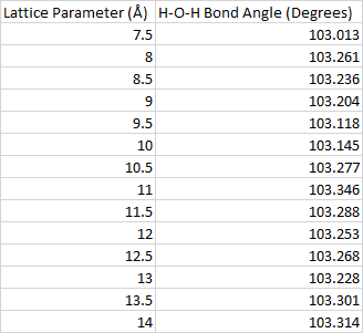
Table A1: H-O-H bond angle as a function of the lattice parameter.

Table A2: H-O-H bond angle as a function of the energy cutoff.

Table A4: Energy of the unoptimized water molecule with respect to the energy cutoff.

Table A3: Energy for the unoptimized water molecule with respect to the lattice parameter.
