Author Archives: Mark Hagemann

Comparison of the Convergence of System Energy and Density of States Calculations with Respect to k-Point Sampling

Purpose of the Calculation

One of the quantities of interest when doing DFT calculations is the electronic density of states (DOS). The DOS is defined as the number of electron states with an energy in the interval E + dE, and is one method for determining the electronic state of the material without examining the full band structure. Our test case for studying the convergence of the DOS will be silver, a metal. The indicative feature of a metal in the DOS is that there are a continuum of available states from below the Fermi energy to above the Fermi energy, which is defined as the energy of the highest energy occupied electron state at zero temperature. This post addresses the topic of properly converging the DOS calculation with respect to k-point mesh, and how that convergence varies from the convergence of the system energy with respect to k-point mesh.

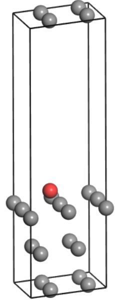
Fig: 1 – The silver unit cell used in this convergence study

Theory of Our Calculation

As with any result that we might report, if we choose to compute the DOS, we must ensure that the result is appropriately converged with respect to the input parameters. To calculate the DOS, we integrate the converged electron density of the system in k-space [1]. Naively, we might then expect that the convergence of the electronic DOS would be similar to the system energy. However, we need to consider the fact that the DOS is a continuous function of energy that needs to be well-resolved for the entire range which we are covering.


The only points at which we calculate the electron density are the points on our k-point mesh. Computationally, we evaluate the integral by doing a weighted sum over the points that we have, using Simpson’s Rule or a similar algorithm. However, when doing something like a Simpson’s Rule algorithm, the function is interpolated in between the points with known values. With a function that rapidly varies in narrow regions, Simpson’s Rule will not give at accurate depiction of the true integral, unless the region is well-sampled. As a result, we should expect that the DOS will not be well-converged without many more k-points than is necessary for the convergence of the energy of the system. We should also expect that this convergence should take the form of the density of states becoming more smoothly varying in the regions where it is non-zero, as the under-sampled regions become appropriately represented.


Calculation Methodology

We use CASTEP [2], a plane-wave basis set package for computing the energies and DOS for our system. Our system is the system depicted in Figure 1, a unit cell of silver atoms on a fcc lattice, with lattice parameter a = 4.086 angstroms. The GGA PBE functional [3] was used for all calculations. The SCF tolerance is 5 x 10^-7 eV, the Koelling-Harmon treatment is used for the atomic solutions [4], and ultrasoft pseudopotentials are generated on the fly. The atoms used in the pseudopotential are 4s2 4p6 4d10 5s1. The integration for the DOS is performed using the 0.2 smearing.


Results

First, a convergence study was performed for the cutoff energy. The results are shown in Figure 2.

Figure 2: Convergence of the system energy with respect to cutoff energy

Above a cutoff energy of 600 eV, the system energy is converged to the order of tenths of an eV, specifically to 0.15 eV. We select 600 eV as the cutoff energy for the rest of our calculations due to being the most computational efficient value converged to this degree. We then calculate both the system energy and the density of states for different k-point meshes. Because our unit cell is cubic, all k-point meshes are of the form NxNxN, where N is an integer, and we will characterize each mesh simply by the number N. Calculations were performed for N=6 to N=20, covering all possible values.


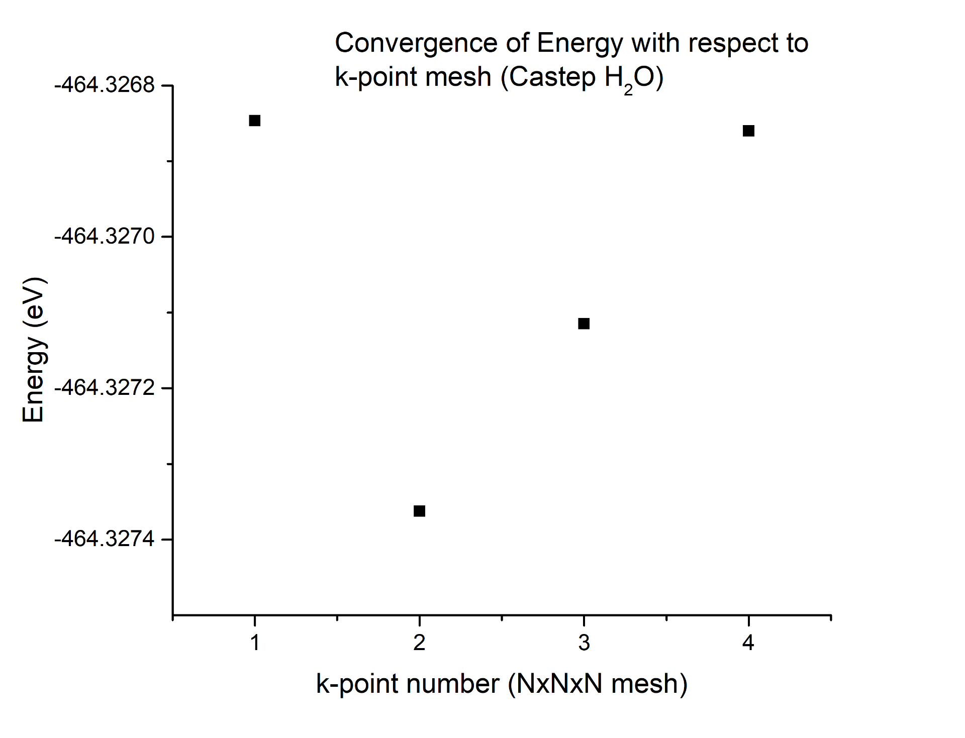
Figure 3: Convergence of the system energy with respect to k-point number

The relevant feature of the convergence results for the system energy with respect to the k-point mesh is that the variance from the 7x7x7 mesh results is never greather than 0.05 eV for higher N, which is already more converged than our results for the cutoff energy. So we can say that our system energy is sufficiently converged at N = 7.

Before comparing the convergence of the DOS, we need to determine a metric for the convergence. It is clear that the behavior of the DOS should qualitatively change in a certain way with an increasing number of k-points, but it is harder to quantitatively measure this change than the change in system energy. We can no longer compare the change in a single value, as the calculated DOS is a curve for each k-point mesh, as show in Figures 4 and 5.

To compare these curves, we take the difference of the DOS value at every point on the curve. We then square these differences, and take the average for each curve. This quantity, defined as (1/N)*Sum(DOS(k, i) – DOS(k-1,i)) is the mean squared deviation between the two DOS curves. Here, N is the number of points on the curve, k or k-1 is the number of points in the k-point mesh used in that DOS calculation, and i is the eV value of a specific point on the curve. The mean squared deviation is a measure of how different two curves are, and minimizing this quantity will imply that the DOS curves are more similar.

Figure 4: The DOS for silver, calculated with a 6x6x6 k-point mesh at 600 eV. The 0 of the x-axis is the Fermi energy.

Figure 5: The DOS for silver, calculated with a 20x20x20 k-point mesh at 600 eV. The 0 of the x-axis is the Fermi Energy.

Because of the extent of the DOS, much of which has no states, we restrict our analysis from eight eV below the Fermi energy to eight eV above the Fermi energy. This portion of the DOS curves are plotted in figures 6 and 7.

Figure 6: The DOS around the Fermi energy for silver, calculated with a 6x6x6 k-point mesh

Figure 7: The DOS around the Fermi energy for silver, calculated with a 20x20x20 k-point mesh

As expected, when the DOS is calculated with a denser sampling of k-space, the curve is smoother and more detailed, rather than sharply varying due to poor sampling.

Quantitatively, as we move from one value of N to the next, the average change in a single point on the curve decreases. It is noteworthy for the some steps in N, there is no change at any point on the DOS curve. This is not indicative of the DOS being fully converged, as shown by later changes to the average deviation. This is representative of the sampling of the new k-point mesh not being significantly different from the previous mesh. The results of this analysis are shown in figures 8 and 9.

Figure 8: Average Squared Difference for the DOS curves with k-mesh specified by N and N-1

Figure 9: Data from figure 8, re-scaled to be more visible

It is noteworthy that these curves are not quite the same as those given in figures 2 and 3. In the case of the system energy, we can simply plot the resulting system energy against k-point number and see the overall trend of the values. We can measure the convergence and fit for behavior at large numbers of k-points. In contrast, we cannot make a truly analogous comparison for the DOS curves.

When we speak about the convergence of the system energy with respect to k-point number, we are addressing the variation between calculation results at a given number of k-points and the result we would obtain with an infinite number of k-points. For a variational parameter, such as the variation of system energy with respect to cutoff energy, this is a relatively easy comparison, since the change in the system energy will always decrease for every additional increase of the energy cutoff by a given amount. For the case of the variation of system energy with respect to k-points, we often test a computationally efficient range of k-points and show that after a certain number of k-points, the system energy does not vary beyond a certain interval, such as 0.05 eV.

In the case of the DOS in this post, we use the mean squared deviation between subsequent curves as a method analogous to comparing variation in the system energy from k-point number to k-point number. The analogous convergence condition is then that the mean squared deviation above a certain number of k-points is below a certain threshold. To facilitate this comparison, we plot the sum of the mean squared deviation in figure 10.

Figure 10: Sum of mean squared deviations for DOS curves. Summed from N=20 back to N=6

Here, we compare the summed mean squared deviation against N=20, our most computationally intensive calculation. This figure makes it clear how the convergence of our calculation proceeds, but we cannot extract predictions about the behavior of the DOS curve at arbitrarily high number of k-points from this figure.

Conclusions

As predicted by the theory, we need many more k-points to appropriately converge the DOS results than we do for the system energy. This should be clear from the clear qualitative differences between figures 6 and 7. More quantitatively, the sum of the mean squared deviations of the DOS curves is approximately 0.005 from N=13 onward. From N=18 onward, the sum of the mean squared deviations is 0.001. If the DOS curve itself is being reported, then the calculation performed at 13x13x13 k-points would give a well-converged result, whereas a lower number of k-points would leave the the sum of the mean squared deviations above 0.18. Meanwhile, the convergence of the system energy with respect to k-points needs only a 6x6x6 k-point mesh.

Additional work in this topic area can investigate the area in an even narrower region around the Fermi energy, which would require an even denser sampling of k-space in that region. This part of the density of states is of particular interest for thermodynamic properties, but is beyond the scope of this post.


References

[1]  D. Sholl and J. Steckel, Density Functional Theory: A Practical Introduction. (Wiley 2009)

[2]  S. J. Clark, M. D. Segall, C. J. Pickard, P. J. Hasnip, M. J. Probert, K. Refson, M. C. Payne, “First principles methods using CASTEP”, Zeitschrift fuer Kristallographie 220(5-6) pp. 567-570 (2005)

[3]  John P. Perdew, Kieron Burke, and Matthias Ernzerhof, “Generalized Gradient Approximation Made Simple”, Phys. Rev. Lett. 77, 3865 – Published 28 October 1996; Erratum Phys. Rev. Lett. 78, 1396 (1997)

[4]  D D Koelling and B N Harmon 1977 J. Phys. C: Solid State Phys. 10 3107

Impact of the Zero Point Energy Correction to Hydrogen Adsorption Sites on the Cu (111) Surface

Purpose of Calculation

In this post, we calculate the zero point energy (ZPE) correction to an adsorbate atom on a surface. The ZPE contributes to the energy of the system, and can affect which binding site on a surface corresponds to the minimum energy arrangement. The ZPE arises from the fact that the adsorbed atom is free to oscillate while still bound to the surface, behaving as a quantum mechanical oscillator. One of the most important features of such an oscillator is, of course, that its lowest energy mode is not a zero energy mode, but a finite energy mode. So, when calculating a system with an adsorbate, we this finite energy (the ZPE) becomes a correction to our calculation. Since the correction energy is the energy of a harmonic oscillator, we expect that the energy should be largely determined by our spring constant (the “stiffness” of our bond” and the mass of the bonded atom. Therefore, the ZPE correction should be most important to atoms such as hydrogen. To demonstrate this, we calculate the ZPE correction for Hydrogen adsorbed at two sites on the Cu (111) surface: the hcp site and the fcc site.

Figure 1: A supercell (2×2) of Hydrogen (red) adsorbed on the (111) surface of copper

Theory of the Zero Point Energy

The ZPE for a quantum mechanical oscillator is given by the sum of the frequencies of the vibrational modes of the system, multiplied by constants. These vibrational modes can be obtained from the eigenvalues of the mass-weighted Hessian matrix of the system. The Hessian matrix is composed of double partial derivatives of the system energy with respect to the displacement of atoms in the system. The energy we calculate for each atomic displacement is in eV, and energy in general relates to time through energy equals mass times distance squared, divided by time squared. The Hessian matrix removes the distance dependence of the Hessian elements. If we then divide out the mass dependence, the elements are in units of inverse seconds squared. If we then take the square root of the eigenvalues of this system, the resulting quantity will be in units of inverse time, as our frequencies should be. In our system, since we are assuming the copper surface’s movement during vibrations will be negligible compared to the hydrogen atom’s movement, the hydrogen atom should be displaced along the x, y, and z direction with an appropriate step size to calculate the second derivatives of energies with respect the movements.

Numerically, we calculate the derivatives using the finite difference approximation. The diagonal elements can be calculated using the first equation below, and the off-diagonal elements can be calculated using the second.[3]

\begin{equation} H_{ii} \cong \frac{E(\delta x_{i})+E(-\delta x_{i})-2E_{0}}{\delta x_{i}^2} \end{equation}
\begin{equation} H_{ij} \cong \frac{E(\delta x_{i}, \delta x_{j})+E(-\delta x_{i},-\delta x_{j})-E(\delta x_{i}, -\delta x_{j})-E(-\delta x_{i}, \delta x_{j})}{4\delta x_{i}\delta x_{j}} \end{equation}


Delta x represents the displacement of the hydrogen atom along direction i or j, and E-naught is the energy when hydrogen is not displaced.

Now, we can diagonalize the Hessian matrix, obtaining the eigenvalues, from which we can directly calculate the vibrational frequencies, using [3]:

\begin{equation} \nu_{i} = \frac{\sqrt{\lambda_{i}}}{2\pi} \end{equation}

where lambda represents the indexed eigenvalue, and nu is the corresponding frequency. These eigenvalues are of the mass-weighted Hessian matrix, which can be obtained be dividing the Hessian matrix by the square root of the mass of the atoms that are being displaced. In our case, this means we should divide by the square root of the mass of hydrogen. Each frequency then contributes an energy

\begin{equation} E_{ZPE} = \frac{h\nu_{i}}{2} \end{equation}

to the ZPE, where h is Planck’s constant.

Calculation Methodology

The ZPE correction to hydrogen on the copper (111) surface is calculated at two sites. For these calculations, we cleave the (111) surface from bulk copper, and then form a super 2×2 supercell, so that both sites are present with all nearest neighbors for interactions. We include three layers of Cu atoms. The lattice parameters are 5.11 angstroms, 5.11 angstroms, 14.17 angstroms (a, b, c). The calculation cell contains 12 unique copper atoms and one unique hydrogen atom. We perform the calculations using Dmol3, which uses a localized basis set [1]. All calculations are performed with the Perdew-Burke-Ernzerhof (PBE) [2] exchange-correlation functional, a Generalized Gradient Approximation (GGA) functional.The on-the-fly basis set is calculated by generating a radial function calculated by solving the density equations on the fly at three hundred points on a logarithmic radial mesh for each atom. This radial function is then multiplied by appropriate spherical harmonics for each atom. We use the DNP basis set method for this calculation. All electrons are included in the Dmol3 calculations. Our SCF threshold is 10^-6 Ha.

We select a 4x4x2 k-point mesh, which test calculations show to be converged to within 0.025 Ha. The cutoff for the localized basis set is set to 4.9 angstroms, and ten angstroms of vacuum space is included in the supercell. We select 0.05 angstroms as our displacement distance. This displacement is selected after calculating the diagonal elements for the Hessian matrix for displacements of 0.01, 0.05 and 0.1 angstroms. 0.01 angstrom displacements did not provide significant changes in the calculated energy relative to the level to which energy was converged. At 0.05 angstroms, there is a significant change in calculated energy, so we elect to use 0.05 angstroms, so that our displacement does not become so large that the finite difference approximation of the derivative is no longer a good approximation.

Results

Calculations were performed for both the hcp and fcc sites with 0.05 angstroms of displacement in each possible combination of directions. Results are shown Table 1.

Displacements (Angstroms)Energy (Ha)
XYZhcpfcc
000-19685.479636-19685.485998
-0.0500-19685.478748-19685.485904
0.0500-19685.480315-19685.485877
0-0.050-19685.480315-19685.485869
00.050-19685.478748-19685.485911
00-0.05-19685.479381-19685.485882
000.05-19685.479387-19685.485759
-0.05-0.050-19685.478283-19685.485797
-0.050-0.05-19685.478244-19685.485762
0-0.05-0.05-19685.479899-19685.485717
-0.050.050-19685.4791136-19685.485798
-0.0500.05-19685.47871-19685.485685
0-0.050.05-19685.477772-19685.485658
0.05-0.050-19685.479407-19685.485774
0.050-0.05-19685.480249-19685.485728
00.05-0.05-19685.479387-19685.485771
0.050.050-19685.479321-19685.485763
0.0500.05-19685.479899-19685.485665
00.050.05-19685.477165-19685.485691

From these values, we can then calculate the appropriate Hessian matrices for each site. As a visual example, the hcp Hessian is

\begin{bmatrix} 8.36\times10^{18} & 9.166\times10^{18} & 8.16\times10^{18} \\ 9.166\times10^{18} & 8.36\times10^{18} & 9.5\times10^{17} \\ 8.16\times10^{18} & 9.5\times10^{17} & 2.016\times10^{19}\end{bmatrix}

Here, all the elements are in units of the square root of mass multiplied by inverse seconds square. Dividing all the elements by square root of the mass of hydrogen and diagonalizing, we obtain the eigenvalues: 5.1258×10^31, 3.1687×10^32 and 6.361×10^32 for the hcp site. For the fcc site, the eigenvalues are 2.0753×10^32, 2.1371×10^32 and 3.4746×10^32. The total ZPE correction for each of these eigenvalues is 0.607 eV for the hcp site and 0.576 eV for the fcc site.

These ZPE corrections are significantly large. Our convergence for the energy calculation, 0.0025 Ha corresponds to approximately 0.068 eV. The corrections are almost an order of magnitude larger than our energy convergence, meaning they represent a correction that should absolutely be included in our calculation. Also of note are that the hcp and fcc corrections differ but hundredths of an eV. When we minimized the energies for each location of the hydrogen atom before displacement, the hcp position was lower than the fcc site by approximately 0.15 eV. As a result, this correction does not change the preferred site from hcp to fcc, but it is still a significant contribution, and illustrates how the ZPE correction can be vital to the proper treatment of systems. With a more stringent convergence of the energy in the calculation, we would be able to better resolve the exact ZPE correction, but at this time, the computational resources were not sufficient to do so in a time-efficient manner.

In addition, possible other sources of error include contributions from copper atoms that Dmol3’s localized basis set do not properly capture, isolation of the hydrogen atom and other similar concerns. In an actual adsorption reaction, there will not be a single hydrogen atom with no other nearby hydrogen on the surface. Instead, something like half the sites might be occupied, or some other, more complex situation. This calculation does not reflect such concerns.

References

[1]  Delley, J., Fast Calculation of Electrostatics in Crystals and Large Molecules; Phys. Chem. 100, 6107 (1996)

[2]  John P. Perdew, Kieron Burke, and Matthias Ernzerhof, “Generalized Gradient Approximation Made Simple”, Phys. Rev. Lett. 77, 3865 – Published 28 October 1996; Erratum Phys. Rev. Lett. 78, 1396 (1997)

[3] D. Sholl and J. Steckel, Density Functional Theory: A Practical Introduction. (Wiley 2009)

Comparing Molecular Geometry Optimization with Localized and non-Localized Basis Sets

Purpose of Calculation

Geometric optimization of a unit cell is useful for finding the minimum energy configuration of a molecule or solid without needing to manually change atom positions. Through numeric minimization algorithms, the proper lattice parameters and atom positions can be obtained. For molecules, this can also find the minimum energy bond angles and bond lengths. However, the different contexts between solids and molecules can present very different challenges. These calculations will compare the convergence and speed of the geometry optimization calculations of water and hydrogen cyanide (HCN), using two different basis sets: Castep’s [1] plane wave basis set and DMol3’s calculated-on-the-fly localized basis set [2].

Figure 1: Optimized geometry of a water molecule

Figure 2: Optimized geometry of a hydrogen cyanide molecule in the H-C-N isomer

Figure 3: Optimized geometry of a hydrogen cyanide molecule in the H-N-C isomer

Calculation Methodology

The bond angle and bond lengths of water and hydrogen cyanide are calculated using two different basis sets.

All calculations are performed with the Perdew-Burke-Ernzerhof (PBE) [3] exchange-correlation functional, a Generalized Gradient Approximation (GGA) functional. The Koelling-Harmon relativistic treatment was used for atomic solutions [4] in the Castep calculations for the plane wave basis set. The on-the-fly basis set is calculated by generating a radial function calculated by solving the density equations on the fly at three hundred points on a logarithmic radial mesh for each atom. This radial function is then multiplied by appropriate spherical harmonics for each atom.

Convergence Calculations

Calculations to check the convergence of the minimum energy output with respect to the energy cutoff, the k-point mesh and the unit cell size were performed for the Castep calculations. It is necessary to check the convergence with respect to the unit cell size because the plane wave basis fills the entire cell. Due to the computational assumption of repeating cells, each unit cell must be large enough so that each molecule does not interact with those in adjacent cells. Convergence tests must be used to idea what is a sufficiently large cell. These tests are shown in figures 4-9 for both water and hydrogen cyanide.


Fig. 4 Convergence of Castep with respect to Cutoff Energy for water

Fig. 5 Convergence of Castep with respect to k-point number for water

Fig. 6 Convergence of Castep with respect to unit cell size for water

Fig. 7 Convergence of Castep with respect to Cutoff Energy for hydrogen cyanide

Fig. 8 Convergence of Castep with respect to k-point number for hydrogen cyanide

Fig. 9 Convergence of Castep with respect to unit cell size for hydrogen cyanide

For DMol3, we do not need to converge the unit cell size. The generated basis sets are highly localized, and we instead test the convergence of the maximum radius of the radial functions, referred to as the cutoff radius. The cutoff radius must be large enough that each atom “sees” the other atoms during all of the geometry optimization, but can still be smaller enough that the basis does not extend as far as the unit cell extends in the Castep calculations. As a result, we check the convergence of energy calculations with respect to cutoff radius and k-point mesh. These convergence tests are shown in figures 10-13 for both water and hydrogen cyanide.

Fig. 10 Convergence of DMol3 with respect to k-point number for water

Fig. 11 Convergence of DMol3 with respect to cutoff radius for water

Fig. 12 Convergence of DMol3 with respect to k-point number for hydrogen cyanide

Fig. 13 Convergence of DMol3 with respect to cutoff radius for hydrogen cyanide

All parameters were converged to within 0.01 eV

Calculation Results

The key metric for comparing the two sets of results is the computational time for both the geometry optimization and the convergence tests. Given an arbitrarily long time, either basis set can give an equally accurate and precise calculation of the bond angles and bond lengths. The important comparison is how quickly the computations can be performed using each basis set to within reasonable agreement with each other.

Both basis sets agree that there is one minimum for the water molecule: a planar bent structure, with bond angle of approximately 104 degrees and a bond length of approximately 0.97 angstroms. Both basis sets also report two isomers of hydrogen cyanide, the H-C-N configuration, and the C-N-H configuration, both with a linear orientation and bond angle of approximately 180 degrees. Disagreement on the exact bond angles and lengths is minor, but does occur. Exact results are included in table one. By better converging the minimum energy, a geometry optimization with a stricter cutoff could be run in order to lessen such disagreement. This, however, is not the purpose of this example case.

BondCastep Bond Length (Angstroms)Castep Bond Angle (Degrees)DMol3 Bond Length (Angstroms)DMol3 Bond Angle (Degrees)
H-O0.9700.971
H-O-H103.708103.708
H-C (H-C-N Isomer)1.0751.076
C-N (H-C-N Isomer)1.1591.164
H-C-N (H-C-N Isomer)175.507179.406
H-N (H-N-C Isomer)1.0061.005
N-C (H-N-C Isomer)1.1761.181
H-N-C (H-N-C Isomer)179.970179.959

The total computation time for both convergence studies and the geometry optimizations for Castep is 8486 seconds (141.43 minutes). For DMol3, the total time is 102 seconds, providing a similar degree of accuracy. This result is expected, due to the more localized basis set being favorable for describing the more local behavior of a molecule confined to a small portion of a cell. The size of the disparity between the two methods is very noteworthy, however, and shows how helpful it can be to choose the correct basis set for a give task.

References

[1]  S. J. Clark, M. D. Segall, C. J. Pickard, P. J. Hasnip, M. J. Probert, K. Refson, M. C. Payne, “First principles methods using CASTEP”, Zeitschrift fuer Kristallographie 220(5-6) pp. 567-570 (2005)

[2]  Delley, J., Fast Calculation of Electrostatics in Crystals and Large Molecules; Phys. Chem. 100, 6107 (1996)

[3]  John P. Perdew, Kieron Burke, and Matthias Ernzerhof, “Generalized Gradient Approximation Made Simple”, Phys. Rev. Lett. 77, 3865 – Published 28 October 1996; Erratum Phys. Rev. Lett. 78, 1396 (1997)

[4]  D D Koelling and B N Harmon 1977 J. Phys. C: Solid State Phys. 10 3107

Determining the Lattice Constants of Hf in an hcp Crystal Structure

Purpose of Calculation

“Hf is experimentally observed to be an hcp metal with c/a = 1.58. Perform calculations to predict the lattice parameters for Hf and compare them with experimental observations.” [1]

Fig. 1 The unit cell for hafnium in the hexagonal close-packed crystal structure

Calculation Methodology

The lattice parameter ratio (c/a) and the lattice constant a are predicted for hafnium in the hcp unit cell, by calculating the minimum energy of the system.

All calculations are performed with the Perdew-Burke-Ernzerhof (PBE) [2] exchange-correlation functional, a Generalized Gradient Approximation (GGA) functional. Pseudopotentials were  calculated on the fly, with the cutoff the 4f electrons and above used as the interacting electrons (4f14 5s2 5p6 5d2 6s2), while lower energy electrons were designated as core electrons (1s2 2s2 2sp 3s2 3p6 3d10 4s2 4p6 4d10). The Koelling-Harmon relativistic treatment was used for atomic solutions. [3]0.1 eV Gaussian smearing was used. Calculations were performed with Castep [4].

Convergence Calculations

Calculations to check the convergence of the minimum energy output with respect to the energy cutoff and the k-point mesh were performed, as shown in figures 2 and 3.

Fig. 2 Convergence calculations of the energy with respect to the k-point number

Fig. 3 Convergence calculations of the energy with respect the energy cutoff

Calculations performed with respect to the energy cutoff were performed with a = 3.1946 angstroms, c = 5.0511 angstroms, and a k-point mesh of 9x9x6. Between 480 eV and 500 eV, the free energy varies less than 0.005 eV, so we select 480 eV as our cutoff energy. Similarly, while varying the k-point mesh, we hold the energy cutoff at 480 eV. At a k-point mesh of 9x9x6, the free energy is similarly converged to 0.005 eV. The remaining calculations were performed at 480 eV and a k-point mesh of 9x9x6.

Calculation Results

Figure 4: Calculation of the internal energy of hcp hafnium as a function of lattice constant a for different ratios of the lattice constants, c/a. Included straight lines are meant to guide the eye and aid in identifying data curves. They do not represent the data themselves.

The minimization of the energy with respect to variation in the lattice constant ratio occurs at c/a = 1.581, which matches experimental observations, and helps support that these calculations are properly converged. The value of a that minimizes the free energy for this ratio is 3.20 angstroms, giving a value of 5.059 angstroms for the predicted value of c. These values for the lattice constants predict the expected unit cell for hafnium in the hcp crystal structure, and agree well with reference values from experiment [5].

References

[1]  D. Sholl and J. Steckel, Density Functional Theory: A Practical Introduction. (Wiley 2009)

[2]  John P. Perdew, Kieron Burke, and Matthias Ernzerhof, “Generalized Gradient Approximation Made Simple”, Phys. Rev. Lett. 77, 3865 – Published 28 October 1996; Erratum Phys. Rev. Lett. 78, 1396 (1997)

[3]  D D Koelling and B N Harmon 1977 J. Phys. C: Solid State Phys. 10 3107

[4]  S. J. Clark, M. D. Segall, C. J. Pickard, P. J. Hasnip, M. J. Probert, K. Refson, M. C. Payne, “First principles methods using CASTEP”, Zeitschrift fuer Kristallographie 220(5-6) pp. 567-570 (2005)

[5]  https://www.webelements.com/hafnium/crystal_structure.html