Most algorithms to identify the Pareto frontier don’t care about the actual values of the points, they only care about the order statistics. Are all of the attributes of one point at least as good as the attributes of another point, and is at least one better? If so, the first point dominates the second. Otherwise not.

So an interesting transformation of the data is to take each column of attributes, and replace their absolute values with a number that indicates their relative position in the ordering. So if we have three points that each have as attributes for max speed as {455, 22, 3090}, we replace those values with {2, 1, 3}. This retains their relative ordering. After doing this for each attribute, you end up with what I call Lattice Latin Hypercube form, or LLH for short. The Mathematica code to generate it is simple:

makeLLH[data_] := Transpose[Map[Ordering[Ordering[#]] &, Transpose[data]]];

Here are some examples of original data and transformed data.

Simplex data

Transformed

Notice how what was originally planar data is now convex. This was a surprise when I first saw it. Next example is spherical data.

Transformed.

Looks very similar. Next up is a rotated rectangular plane

Here’s a rotating GIF so you can see it is transformed from planar to…something otherwise. Click on the image to see it rotate, unable to do so in the post.

 

Here’s 4000 pts distributed multi-variate normal on a plane, and the transformed version. Significant difference!

Click on the plot to see a rotation.

 

If you are going to talk Pareto Frontier, you ought to know something about the simplex, in particular a right-simplex or orthogonal simplex. It is the simplest geometric figure you can construct in a particular dimensional space. There is of course a Wikipedia page full of useful information:

http://en.wikipedia.org/wiki/Simplex

What I will talk about here are the particular aspects that I find useful in analyzing Pareto Frontiers. First some definitions and laying out of terms.

So what exactly is a simplex? It is the simplest geometric figure possible within a particular dimensional space. This is a triangle in 2D space (three points), a tetrahedron in 3D space, and so on.

The geometric figure below is a trirectangular tetrahedron. The red face is referred to as the base facet, and the vertex opposite the base facet is the peak vertex. It is trirectangular because the three edges touching the base facet intersect at right angles to each other. For this case, the lengths of the edges that meet at the peak vertex are all the same length.

As noted, the d-dimensional generalization of a tetrahedron is the simplex. Referring to a simplex in d dimensions as a d-simplex, it will have d+1 facets, with each facet being a (d-1)-simplex itself. For example, the tetrahedron above is a simplex in 3D space, it has 3+1=4 facets, and each facet is a triangle, which is just a simplex in 2D space.

A d-dimensional simplex will be referred to as a d-rectangular simplex if all edges emanating from the peak vertex are orthogonal to each other, which is the case here. For this work, the lengths of the edges extending from the peak vertex are equal to each other, resulting in a higher dimensional analog to a right triangle referred to as a d-right simplex.

For labeling, we will refer to the edge length as l and the shortest distance from the apex to the base facet as q, as per the picture below.

The generalized term for the volume (3D) or area (2D) is the content. For a d-right simplex with orthogonal edges of length l, the content  c is

$$c=\int _0^l\int _0^{x_1}\int _0^{x_2}…\int _0^{x_{d-1}}dx_d…dx_3dx_2dx_1$$

or

$$c=\frac{l^d}{d!}$$

The relationship between edge length l and the distance q from the peak to the base facet is

$$q=\frac{l}{\sqrt{d}}$$

The generalized pythagorean theorem says that the square of the content of the base facet is the sum of the contents of the of the other (side) facets, and so

$$c_b^2=\sum _d c_s^2=d c_s^2$$

Since the content of the side facets is

$$c=\frac{l^{d-1}}{d-1!}$$

The content of the base facet is

$$c=\sqrt{d}\frac{l^{d-1}}{d-1!}$$

A little more massaging to get the area of the base facet in terms of q gives us

$$c_b=\frac{d^{d/2}} {d-1!}q^{d-1}$$

or defining the parameter α which is only a function of d:

$$\alpha _d=\frac{d^{d/2}}{d-1!}$$

We end up with the final version…

$$c_b=\alpha _d q^{d-1}$$

With this information, we can reason about relationships between clouds of Pareto points on the base facet and their dominated hypervolume. This, for a future post.

OK, experimenting with how to make blog entries, and also providing some information on how to generate points that are all Pareto optimal but are otherwise as random as possible. I created these methods back in 2004 while working on my PhD thesis. Since then, they’ve been recreated many times over, and one can google on them and get lots of hits. Here’s a useful page.

http://stackoverflow.com/questions/3010837/sample-uniformly-at-random-from-an-n-dimensional-unit-simplex

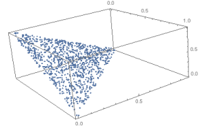
The algorithm to generate points on a simplex

Here’s a picture of 1000 points in 3 dimensions.

Here’s the code. If you cut and paste this into Mathematica, you may need to delete and retype the “d-1” term, as some sort of hidden formatting seems to carry over and mess up the evaluation when I try it.

genSimplex[n_, d_] := Table[Differences[Sort[Flatten[{0, RandomReal[1, d – 1], 1}]]], {n}];

The algorithm generates points that are randomly distributed on an outer face of a simplex. The way to generate them is, for a d-dimensional problem…

1. Generate d-1 uniformly distributed random values in the range [0,1]
2. Add a 0 and a 1 to the list
3. Sort the list
4. Extract a list of the differences between the elements

You now have a list of random values that sum to 1 (so they are on a plane that is defined by points that sum to one) and that are otherwise independent of each other, so their dispersion is uniform.

Generating Points on Hypersphere

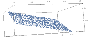
This algorithm uses the fact that multivariate normal points distributed with \[Mu] = {0,…,0} and \[CapitalSigma] = Identity Matrix are uniformly sprayed out in all directions. So generate the points, take the absolute value of the coordinate values to move them all to the positive quadrant, and then normalize them to project them onto the unit hypersphere.

genSphere[n_, d_] := Table[Normalize[Abs[RandomVariate[MultinormalDistribution[ConstantArray[0, d], IdentityMatrix[d]]]]], {n}]

Picture of 1000 pts in 3D, with the aspect ratio a little squashed.

 

Generating Points on a Plane And Then Rotating Them

This algorithmic approach first generates points that form a d-1 dimensional cloud embedded in d dimensions, so each point has value [0  x1  x2 …. xd]. Thus the points are on a plane orthogonal to a d-dimensional vector [1  0 …. 0]. We next create a rotation matrix that will rotate the vector to [1 1 1 …. 1], and orthogonalize it. We then just multiply each of the data points by this matrix.

First example is generating a could that is distributed uniformly over a d-1 hypercube.

genRotatedPlane[n_, d_] := Map[Transpose@Orthogonalize@ReplacePart[IdentityMatrix[d], {1, i_} -> 1].# &, Transpose@Prepend[RandomReal[1, {d – 1, n}], Array[0 &, n]]];

You may need to retype sections in case some odd hidden formatting carries through. Example data set, 1000 pts in 3D.

 

 

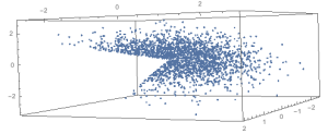
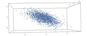
Similar to above, but rather than generating a d-1 hypercube, we generate a d-1 multi-variate normal cloud with μ = [0 0 … 0] and Σ as the identity matrix. Lots of other potential approaches to generating the initial data prior to rotation.

genRotatedPlaneNormal[n_, d_] :=
Map[Transpose@Orthogonalize@ReplacePart[IdentityMatrix[d], {1, i_} -> 1].# &, Transpose@Prepend[RandomVariate[NormalDistribution[], {d – 1, n}], Array[0 &, n]]];

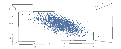
Here’s a modification that removes a chunk of the data.

genRotatedPlaneNormalChunkMissing[n_, d_] :=
Map[Transpose@Orthogonalize@ReplacePart[IdentityMatrix[d], {1, i_} -> 1].# &,
Select[Transpose@Prepend[RandomVariate[NormalDistribution[], {d – 1, n}],
Array[0 &, n]], ! AllTrue[#, NonPositive] &]];