
Introduction
In this post we calculate the vibrational frequencies and zero point energy (ZPE) of a hydrogen absorbed on the surface of Cu(111). This is done by first doing geometry optimization to find the preferred location of the hydrogen atom in the hcp or fcc interstitial site. After this, the hydrogen atom is perturbed from the energy minimum in increments of 0.05 Å in order to calculate the hessian matrix. The mass-weighted hessian matrix is then diagonalized to find the vibrational frequencies and thus the ZPE of the hydrogen atom.
Surface Construction
The surface of the Cu(111) with hydrogen adsorbents is modeled with 4 layers of Cu(111) and hydrogen atoms at the corresponding hcp interstitial sites on each side as seen in fig 1.
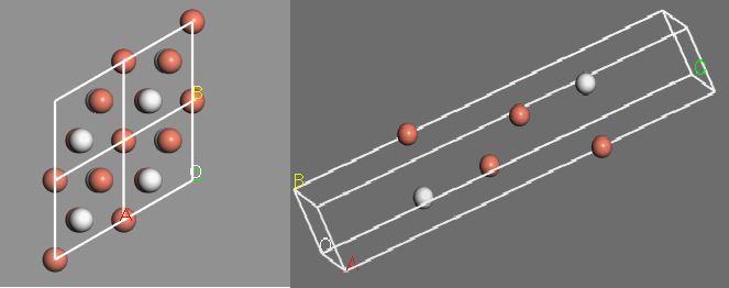
Fig. 1: Top view of hydrogen in the hcp interstitial site on the Cu(111) surface with periodic boundary conditions (left). Side view of the slab model with hydrogen in the hcp site (right).
The Cu(111) slab along with the hydrogen atoms is then centered within a vacuum slab that is 15 Å thick.
Details of the Calculations
All calculations were performed with the CASTEP package in materials studio with the GGA Perdew-Burke-Ernzerhof functional [1-2]. The pseudopotential was solved with the Koelling-Harmon atomic and 1s2 2s2 2p6 3s2 3p6 for the inner shells, while 3d10 4s1 were used for the outer shells.
Geometry optimization calculations used convergence tolerances of 10^-5 eV/atom, 0.03 eV/Å for the max force, 0.05 GPa for the max stress, and a max displacement of 0.001 Å. A rough calculation using an energy cutoff of 408 eV and a 6x6x1 k-point set is performed to get an idea of where the hydrogen atoms will relax to. After this, the energy cutoff and the number of k-points are increased until there is less than a 0.01 eV change in the system energy. A geometry optimization is then performed again to find the final location of the hydrogen atoms. Through this procedure we find that an energy cutoff of 480 eV and a 12x12x2 k-point set, corresponding to 144 inequivalent k-points is found to be acceptable.
We are then able to calculate energies around the minimum by slightly perturbing the hydrogen atoms from their preferred positions. Shifting a hydrogen direction in one direction on one surface corresponds to a shift in the opposite direction on the other surface in order to preserve the symmetry of the system. The results of these calculations for the hcp site are shown in table 1, and the results for the fcc site are shown in table 2.
| dx (Å) | dy (Å) | dz (Å) | Energy (eV) |
|---|---|---|---|
| 0 | 0 | 0 | -6753.163 |
| 0.05 | 0 | 0 | -6753.151 |
| -0.05 | 0 | 0 | -6753.147 |
| 0 | 0.05 | 0 | -6753.152 |
| 0 | -0.05 | 0 | -6753.152 |
| 0 | 0 | 0.05 | -6753.150 |
| 0 | 0 | -0.05 | -6753.153 |
| 0.05 | 0.05 | 0 | -6753.143 |
| 0.05 | 0 | 0.05 | -6753.141 |
| 0 | 0.05 | 0.05 | -6753.142 |
| 0.05 | -0.05 | 0 | -6753.143 |
| 0.05 | 0 | -0.05 | -6753.141 |
| 0 | 0.05 | -0.05 | -6753.141 |
| -0.05 | 0.05 | 0 | -6753.140 |
| -0.05 | 0 | 0.05 | -6753.142 |
| 0 | -0.05 | 0.05 | -6753.142 |
| -0.05 | -0.05 | 0 | -6753.140 |
| -0.05 | 0 | -0.05 | -6753.142 |
| 0 | -0.05 | -0.05 | -6753.141 |
| dx (Å) | dy (Å) | dz (Å) | Energy (eV) |
|---|---|---|---|
| 0 | 0 | 0 | -6753.134 |
| 0.05 | 0 | 0 | -6753.124 |
| -0.05 | 0 | 0 | -6753.123 |
| 0 | 0.05 | 0 | -6753.124 |
| 0 | -0.05 | 0 | -6753.124 |
| 0 | 0 | 0.05 | -6753.123 |
| 0 | 0 | -0.05 | -6753.124 |
| 0.05 | 0.05 | 0 | -6753.112 |
| 0.05 | 0 | 0.05 | -6753.115 |
| 0 | 0.05 | 0.05 | -6753.115 |
| 0.05 | -0.05 | 0 | -6753.112 |
| 0.05 | 0 | -0.05 | -6753.113 |
| 0 | 0.05 | -0.05 | -6753.112 |
| -0.05 | 0.05 | 0 | -6753.115 |
| -0.05 | 0 | 0.05 | -6753.114 |
| 0 | -0.05 | 0.05 | -6753.115 |
| -0.05 | -0.05 | 0 | -6753.114 |
| -0.05 | 0 | -0.05 | -6753.111 |
| 0 | -0.05 | -0.05 | -6753.112 |
Calculation of Frequencies and Zero Point Energies
The Hessian matrix, \(\frac{\partial^2 E}{\partial x_i \partial x_j}\), can be approximated using the data in table 1. We approximate the diagonal terms with
\[\frac{\partial^2 E}{\partial x_i \partial x_i} = \frac{E(x_i + \Delta x_i) – 2E(x_i) + E(x_i – \Delta x_i)}{\Delta x_i^2}\]
and the off-diagonal terms with
\[\frac{\partial^2 E}{\partial x_i \partial x_j} = \frac{E(x_i + \Delta x_i, x_j + \Delta x_j) – E(x_i + \Delta x_i, x_j – \Delta x_j) – E(x_i – \Delta x_i, x_j + \Delta x_j) + E(x_i – \Delta x_i, x_j – \Delta x_j)}{4 \Delta x_i \Delta x_j}\].
To convert to the mass-weighted Hessian, we can simply divide by the mass of the hydrogen atoms. We divide by 2 times the mass in order to account for both atoms. The frequencies are then given by \(\nu_i = \frac{\sqrt{\lambda_i}}{2 \pi}\), where \(\lambda_i\) are the eigenvalues of the mass-weighted Hessian matrix.
Through this procedure we obtain vibrational frequencies of 36.9 THz, 32.7 THz, and 33.4 THz. We can then calculate the ZPE by treating these frequencies as those corresponding to ground states of independent quantum harmonic oscillators:
\[E_{ZPE} = \sum\limits_{i} \frac{\hbar \omega_i}{2}\]
This gives a ZPE of 0.213 eV for the hydrogen in the hcp interstitial site.
For the fcc site, this same procedure gives vibrational frequencies of 32.1 THz, 31.8 THz, and 31.1 THz. These correspond to a ZPE of 0.196 eV
Conclusions
In this post, we constructed a Cu(111) surface with hydrogen adsorbed onto either the hcp or fcc interstitial sites. We then performed geometry optimization and calculated the energies of the system when the hydrogen atoms were perturbed slightly from their minima. This allowed us to calculate the mass-weighted Hessian matrix, which was then diagonalized to give the vibrational frequencies and thus the zero-point energies. Without the inclusion of zero-point energies, the system with fcc defects is higher in energy by 0.029 eV. With the inclusion of zero-point energies, this system is greater in energy by 0.012 eV.
References
1.) First principle methods using CASTEP Zeitschrift fuer Kristallographie 220(5-6) pp. 567-570 (2005).
2.) Perdew, J.P., K. Burke, and M. Ernzerhof, Generalized gradient approximation made simple.Physical review letters, 1996. 77(18): p. 3865.
