Author Archives: Garrett DuCharme

Hopping of Hydrogen on the Surface of Cu(111): A Transition State Study

Introduction

This post will focus on applying transition state theory to hydrogen atoms adsorbed onto the surface of Cu(111). We first use geometry optimization to find the preferred position of hydrogen on the FCC and HCP sites on the Cu(111) surface. After this, transition state calculations using the complete linear synchronous transit and quadratic synchronous transit (LST/QST) method are performed in order to find the energy barriers [1].

The Slab Model and Geometry Optimization

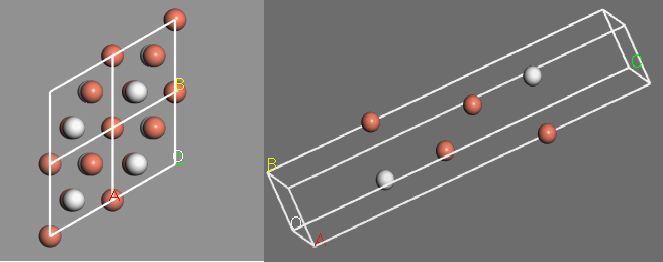
We use a slab model consisting of 4 layers of Cu and a single hydrogen atom adsorbed to the surface. The vacuum is chosen to be 10 Å thick, and the lattice vectors are (2.21 Å, -1.28 Å, 0), (0, 2.56 Å, 0), and (0, 0, 16.26 Å).

Fig 1: The slab model for Cu(111) with a hydrogen adsorbed onto the surface.

All calculations were performed with the CASTEP package in materials studio with the GGA Perdew-Burke-Ernzerhof functional [2-3]. The pseudopotential was solved with the Koelling-Harmon atomic and 1s2 2s2 2p6 3s2 3p6 for the inner shells, while 3d10 4s1 were used for the outer shells.

Geometry optimization calculations used convergence tolerances of 10^-5 eV/atom, 0.03 eV/Å for the max force, 0.05 GPa for the max stress, and a max displacement of 0.001 Å. The k-point set is increase from 6x6x1 to 10x10x1, and then from 10x10x2 to 12x12x2 to test for convergence. In changing to k-point set from 12x12x2 to 13x13x2, there is less than a 0.01 eV change in the system energy. Convergence for the cutoff energy is tested by starting at 440 eV and increasing until 570 eV. This test shows that there is less than a 0.01 eV change in the energy when going from 480 eV to 490 eV.

Fig 2: Test of the convergence for the cutoff energy. An identical trend is observed for hydrogen at the HCP site.

Transition State Calculations

The trajectory for the hydrogen transition was predicted using the Materials Studio “reaction preview” tool.

Fig 3: Side view of hydrogen moving from the HCP site to the FCC site on the surface of Cu(111) as determined by the reaction preview tool.

Fig 4: Top-down view of hydrogen moving from the HCP site to the FCC site on the surface of Cu(111) as determined by the reaction preview tool.

The transition state and energy barrier are then calculated using the LST/QST method. The RMS convergence is chosen to be 0.05 eV/Å with the maximum number of QST steps set to 5. Calculations were done to show that the energy barriers are converged well for changes of 20 eV to the energy cutoff for cutoffs past 480 eV. The reaction pathway and the energies are shown in fig 4. The transition state is found to have an energy of -6736.2477 eV.

Table 1: Variation of the energy barriers with increasing energy cutoff.

Fig 4: Reaction pathway for a hydrogen jumping from the HCP site to the FCC site. The blue star indicates the position of the transition state.

We have previously found that the hydrogen atom at the HCP site has vibrational frequencies of 36.9 THz, 32.7 THz, and 33.4 THz, while at the FCC site it has vibrational frequencies of 32.1 THz,  31.8 THz, and  31.1 THz. We can once again apply the Hessian matrix method to find the vibrational frequencies for the transition state. These frequencies give zero-point energy corrections of 0.213 eV and 0.196 eV, respectively.

Table 2: Perturbations in the energy for small changes in the hydrogen atom position at the transition state. These are used to calculate the Hessian matrix.

Doing this, we find that the transition state has real frequencies of 63.2 Thz and 32.0 THz. There is one imaginary frequency of 23.0 Thz, which corresponds to the hydrogen moving from the HCP site to the FCC site or vice-versa. The corresponding zero-point energy correction is then 0.197 eV.

Using the zero-point energy corrections, we can then find the corrections to the energy barriers. This correction is defined as

\[\Delta E_{ZP} = \bigg( E^{\dagger} + \sum_{j=1}^{N-1} \frac{h \nu_{j}^{\dagger}}{2} \bigg) – \bigg( E_{A} + \sum_{i=1}^{N} \frac{h \nu_{i}^{\dagger}}{2} \bigg) \]

Here, \(E^{\dagger} \) is the energy of the transition state and \(E_{A} \) is the energy in either the HCP site or the FCC site. The sum with j sums over the N-1 real modes at the transition state, while the sum over i sums over the normal modes in either the FCC or HCP site. These two sums simply give the zero point energy corrections that we have calculated above.

For a transition with hydrogen starting in the HCP site, the energy barrier will be corrected to 0.230 eV. For a transition from the FCC site, the correction to the energy barrier is 0.219 eV.

Conclusions

Using transition state theory, we find that hydrogen hopping from the HCP to FCC vacancy site on the surface of Cu(111) has an energy barrier of 0.247 eV, while hopping in the other direction has an energy barrier of 0.220 eV. Using the zero-point energy correction, we find that these barriers are corrected to 0.230 eV and 0.219 eV, respectively. These correspond to 4.3% and 0.5% changes from the original energy barriers.


References

[1] Govind, N., Petersen, M., Fitzgerald, G., King-Smith, D., & Andzelm, J. (2003). A generalized synchronous transit method for transition state location. Computational Materials Science,28(2), 250-258.

[2] First principle methods using CASTEP Zeitschrift fuer Kristallographie 220(5-6) pp. 567-570 (2005).

[3] Perdew, J.P., K. Burke, and M. Ernzerhof, Generalized gradient approximation made simple.Physical review letters, 1996. 77(18): p. 3865.

Vibrational Frequencies and Zero Point Energies of Hydrogen on the surface of Cu(111)

Introduction

In this post we calculate the vibrational frequencies and zero point energy (ZPE) of a hydrogen absorbed on the surface of Cu(111). This is done by first doing geometry optimization to find the preferred location of the hydrogen atom in the hcp or fcc interstitial site. After this, the hydrogen atom is perturbed from the energy minimum in increments of 0.05 Å in order to calculate the hessian matrix. The mass-weighted hessian matrix is then diagonalized to find the vibrational frequencies and thus the ZPE of the hydrogen atom.

Surface Construction

The surface of the Cu(111) with hydrogen adsorbents is modeled with 4 layers of Cu(111) and hydrogen atoms at the corresponding hcp interstitial sites on each side as seen in fig 1.

Fig. 1: Top view of hydrogen in the hcp interstitial site on the Cu(111) surface with periodic boundary conditions (left). Side view of the slab model with hydrogen in the hcp site (right).

The Cu(111) slab along with the hydrogen atoms is then centered within a vacuum slab that is 15 Å thick.

Details of the Calculations

All calculations were performed with the CASTEP package in materials studio with the GGA Perdew-Burke-Ernzerhof functional [1-2]. The pseudopotential was solved with the Koelling-Harmon atomic and 1s2 2s2 2p6 3s2 3p6 for the inner shells, while 3d10 4s1 were used for the outer shells.

Geometry optimization calculations used convergence tolerances of 10^-5 eV/atom, 0.03 eV/Å for the max force, 0.05 GPa for the max stress, and a max displacement of 0.001 Å. A rough calculation using an energy cutoff of 408 eV and a 6x6x1 k-point set is performed to get an idea of where the hydrogen atoms will relax to. After this, the energy cutoff and the number of k-points are increased until there is less than a 0.01 eV change in the system energy. A geometry optimization is then performed again to find the final location of the hydrogen atoms. Through this procedure we find that an energy cutoff of 480 eV and a 12x12x2 k-point set, corresponding to 144 inequivalent k-points is found to be acceptable.

We are then able to calculate energies around the minimum by slightly perturbing the hydrogen atoms from their preferred positions. Shifting a hydrogen direction in one direction on one surface corresponds to a shift in the opposite direction on the other surface in order to preserve the symmetry of the system. The results of these calculations for the hcp site are shown in table 1, and the results for the fcc site are shown in table 2.

dx (Å)dy (Å)dz (Å)Energy (eV)
000-6753.163
0.0500-6753.151
-0.0500-6753.147
00.050-6753.152
0-0.050-6753.152
000.05-6753.150
00-0.05-6753.153
0.050.050-6753.143
0.0500.05-6753.141
00.050.05-6753.142
0.05-0.050-6753.143
0.050-0.05-6753.141
00.05-0.05-6753.141
-0.050.050-6753.140
-0.0500.05-6753.142
0-0.050.05-6753.142
-0.05-0.050-6753.140
-0.050-0.05-6753.142
0-0.05-0.05-6753.141
Table 1: Calculations of the system energies for perturbations of the hydrogen atoms about their minima in the hcp interstitial site.
dx (Å)dy (Å)dz (Å)Energy (eV)
000-6753.134
0.0500-6753.124
-0.0500-6753.123
00.050-6753.124
0-0.050-6753.124
000.05-6753.123
00-0.05-6753.124
0.050.050-6753.112
0.0500.05-6753.115
00.050.05-6753.115
0.05-0.050-6753.112
0.050-0.05-6753.113
00.05-0.05-6753.112
-0.050.050-6753.115
-0.0500.05-6753.114
0-0.050.05-6753.115
-0.05-0.050-6753.114
-0.050-0.05-6753.111
0-0.05-0.05-6753.112
Table 1: Calculations of the system energies for perturbations of the hydrogen atoms about their minima in the fcc interstitial site.

Calculation of Frequencies and Zero Point Energies

The Hessian matrix, \(\frac{\partial^2 E}{\partial x_i \partial x_j}\), can be approximated using the data in table 1. We approximate the diagonal terms with

\[\frac{\partial^2 E}{\partial x_i \partial x_i} = \frac{E(x_i + \Delta x_i) – 2E(x_i) + E(x_i – \Delta x_i)}{\Delta x_i^2}\]

and the off-diagonal terms with

\[\frac{\partial^2 E}{\partial x_i \partial x_j} = \frac{E(x_i + \Delta x_i, x_j + \Delta x_j) – E(x_i + \Delta x_i, x_j – \Delta x_j) – E(x_i – \Delta x_i, x_j + \Delta x_j) + E(x_i – \Delta x_i, x_j – \Delta x_j)}{4 \Delta x_i \Delta x_j}\].

To convert to the mass-weighted Hessian, we can simply divide by the mass of the hydrogen atoms. We divide by 2 times the mass in order to account for both atoms. The frequencies are then given by \(\nu_i = \frac{\sqrt{\lambda_i}}{2 \pi}\), where \(\lambda_i\) are the eigenvalues of the mass-weighted Hessian matrix.

Through this procedure we obtain vibrational frequencies of 36.9 THz, 32.7 THz, and 33.4 THz. We can then calculate the ZPE by treating these frequencies as those corresponding to ground states of independent quantum harmonic oscillators:

\[E_{ZPE} = \sum\limits_{i} \frac{\hbar \omega_i}{2}\]

This gives a ZPE of 0.213 eV for the hydrogen in the hcp interstitial site.

For the fcc site, this same procedure gives vibrational frequencies of 32.1 THz, 31.8 THz, and 31.1 THz. These correspond to a ZPE of 0.196 eV

Conclusions

In this post, we constructed a Cu(111) surface with hydrogen adsorbed onto either the hcp or fcc interstitial sites. We then performed geometry optimization and calculated the energies of the system when the hydrogen atoms were perturbed slightly from their minima. This allowed us to calculate the mass-weighted Hessian matrix, which was then diagonalized to give the vibrational frequencies and thus the zero-point energies. Without the inclusion of zero-point energies, the system with fcc defects is higher in energy by 0.029 eV. With the inclusion of zero-point energies, this system is greater in energy by 0.012 eV.


References

1.) First principle methods using CASTEP Zeitschrift fuer Kristallographie 220(5-6) pp. 567-570 (2005).

2.) Perdew, J.P., K. Burke, and M. Ernzerhof, Generalized gradient approximation made simple.Physical review letters, 1996. 77(18): p. 3865.

Exploring Geometry Optimization with a Water Molecule

Introduction

The focus of this post will be to explore different aspects of geometry optimization by studying a water molecule. The most stable geometry of water has an O-H bond length of 0.957 Å and an H-O-H bond angle of 104.2° [1]. We will use this fact to test various parameters of the simulation. The geometry optimization calculations were done with the CASTEP density functional theory (DFT) package in Materials Studio [2]. The CASTEP plane wave basis set requires periodic boundary conditions, which creates issues when studying a single molecule. One must carefully consider the size of the simulation cell being used so that the periodic images of the molecule, as seen in fig. 1, do not interact.

Fig. 1: A single water molecule and some of its periodic images.

All calculations use the GGA with the PBE functional [3]. Atomic and pseudo atomic calculations for hydrogen both use the 1s1 electron. Atomic calculations for oxygen are done for the 1s2 2s2 2p4 electrons, while the pseudo atomic calculations are done for the 2s2, 2p4 electrons. The SCF tolerance is 5.0*10^-7 eV/atom and the convergence tolerance is set to 5.0*10^-6 for energy, 0.01 eV/Å for the max force, 0.02 GPa for the max stress, and 5.0*10^-4 Å for the maximum displacement. Unless otherwise specified, the initial conditions are chosen so that the oxygen atom is centered at the origin, while the two hydrogen atoms are at positions (0, 0.707 Å, 0.707 Å) and (0, 0.707 Å, -0.707 Å), giving an initial bond length of 1 Å and an H-O-H angle of 90°.

The rest of the post will be organized into sections focused on understanding the effects of the unit cell size, the energy cutoff, the k-space sampling, variations of the initial conditions, and a discussion of the final results.

Unit Cell Size

The calculations are done with a cubic unit cell. In order to understand the effects that the images have on each other, we vary the lengths of the cube sides from 7.5 Å to 14 Å in increments of 0.5 Å. Each one of these calculations is done with just the gamma k-point and an energy cutoff of 400 eV.

Fig. 2: Variation of the H-O-H bond angle with respect to the lattice parameter.

By looking at the H-O-H bond angle, we can get an idea of how big the unit cell needs to be in order to minimize the role that the images play in the geometry optimization. Fig. 2 shows that this angle changes rapidly at first, but then starts to stabilize at around 12 Å. A table of the data seen in this plot can be found in the appendix. Unit cells with lattice parameters larger than 12 Å take longer to converge, so this is the lattice parameter that will be chosen for the rest of the calculations.

In order to further confirm that this is an appropriate unit cell size, we can also check to see if the energy has converged.

Fig. 3: Energy of the unoptimized water molecule vs the lattice parameter.

The energy changes by less than 0.1 eV once the lattice parameter is greater than 9 Å. Exact values for these calculations are provided in the appendix.

Energy Cutoff

The calculations for testing the energy cutoff were again done with a k-space sampling that only includes the gamma point. We observe changes in the H-O-H bond angle in increments of 20 eV from 400 eV to 660 eV. A table of these calculations can be found in the appendix.

Fig. 4: Variation of the H-O-H bond angle with respect to the energy cutoff.

As can be seen in fig. 3, the H-O-H bond angle does not have any significant change past an energy cutoff of 600 eV.

We can once again further verify that this is an acceptable energy cutoff by looking at the energy of the unoptimized water molecule as we increase the energy cutoff.

Fig. 5: Energy of the unoptimized water molecule vs the energy cutoff.

The energy changes by less than 0.1 eV between an energy cutoff of 560 eV and 600 eV. Exact values for the energies can be found in the appendix.

K-space Sampling

Due to the high symmetry and size of the unit cell, one should expect that the k-space sampling will have little to no impact on the final geometry of the water molecule centered at the origin in real space. We observe that there is no change in the H-O-H bond angle when using 1, 4, or 14 k-points for energy cutoffs of 400 eV as well as 600 eV.

Testing Initial Conditions

Different initial conditions, i.e the initial bond lengths and the bond angles, provide insight into how the geometry optimization is performed. Given a sufficiently large box size and energy cutoff, one would expect that the water molecule should always converge to the optimal geometry regardless of the initial conditions because it has only one stable configuration. For more complicated molecules, it is important to consider the possibility that there are other stable isomers.

Table 1: Effects of initial conditions on the final geometry of the water molecule and the number of optimization steps. All calculations are run with a lattice parameter of 12 Å and an energy cutoff of 600 eV with only the gamma k-point.

The results in table 1 show that starting with an initial angle of 180° will only cause a change in the two bond lengths. This is because the forces between the atoms only need to be minimized along a line instead of within a plane. Furthermore, we see that starting with two different bond lengths will cause the optimization procedure to take longer to achieve the same result. One can see that achieving what appears to be the most physical result in the shortest amount of steps requires the two initial bond lengths to be the same, while the initial angle must be less than 180°.

Discussion

In order to have accurate geometry optimization calculations of molecules with a plane wave basis set, the chosen unit cell must be sufficiently large so that images of the molecule do not interact. Furthermore, it is important that the cell not be arbitrarily large such that the computation time becomes unreasonable. Once this parameter has been tested, investigations into a suitable energy cutoff can be performed. Convergence can be tested yet again by varying the number of k-points. For a small molecule such as water, just the gamma point was shown to be sufficient. Finally, by utilizing symmetries in the system it is possible to decrease the number of optimization steps. However, one must be careful to make sure that the final results are physical, and to also explore the possibility of other stable isomers.

References

  1.  Hoy, A. R. & Bunker, P. R. A precise solution of the rotation bending Schrödinger equation     for a triatomic molecule with application to the water molecule. Journal of Molecular                 Spectroscopy 74, 1–8 (1979).
  2.  Clark, S. et al. First principles methods using CASTEP. Z. Kristallogr. 220, 567–570 (2005).
  3.  Perdew, J. P; Burke, K; Ernzerhof, M. Phys. Rev. Lett. 1996, 77, 3865-3868.

Appendix

Table A1: H-O-H bond angle as a function of the lattice parameter.

Table A2: H-O-H bond angle as a function of the energy cutoff.

Table A4: Energy of the unoptimized water molecule with respect to the energy cutoff.

Table A3: Energy for the unoptimized water molecule with respect to the lattice parameter.

Determination of Structure and Lattice Constant for Platinum

Overview of the Problem

This post will be about determining both the structure and lattice constant for platinum. This will be done using density functional theory (DFT) to calculate the cohesive energies across a range of lattice parameters for platinum in the simple cubic (SC), face-centered cubic (FCC), and hexagonal close-packed (HCP) structures.

In order to make sure the results are feasible, convergence tests are first done for both the number of k-points and the cutoff energies.

All calculations are done in Materials Studio with the CASTEP DFT package [1]. The functional used was that of Perdew Burke Ernzerhof [2], and the pseudopotential was obtained using the Koelling-Harmon solver for the 4f14 5s2 5p6 5d9 6s1 outer shells. 

Cutoff Energy Convergence

The cutoff energy was tested by starting at a cutoff energy of 360 eV and then increasing by increments of 30 eV to look for convergence in the free energy. For this test the lattice parameters of the three structures were chosen as a = 3.92 Å for FCC, a = 2.62 Å for SC, and a = 3.02 Å, c = 4.83 Å for HCP. These lattice constants were chosen for this test by roughly estimating the location of the minimum of the three structures at an energy cutoff of 300 eV. The results are outlined in table 1 and figure 1.


Energy Cutoff (eV)FCC Free Energy (eV)SC Free Energy (eV)HCP Free Energy (eV)
300-13050.818-13050.421-13049.923
330-13050.927-13050.534-13050.046
360-13050.960-13050.568-13050.080
390-13050.970-13050.578-13050.116
420-13050.973-13050.580-13050.119
450-13050.973-13050.581-13050.120
480-13050.974-13050.581-13050.120
510-13050.974-13050.581-13050.120
Table 1: Data for the energy cutoff convergence test.

As can be seen from the figure and the table, a lower energy cutoff here will overestimate the free energy. It can also be see that the variation in the free energy is less than 0.01 eV past the 390 eV cutoff energy. For consistency, a cutoff energy of 420 eV has been chosen for all calculations involving the determination of the lattice parameters.

K-Point Convergence

The k-point convergence was tested using an HCP structure with a = 3.12 Å and c/a = 1.6, an SC structure with a = 2.62 Å, and an FCC structure with a = 3.92 Å. The results are outlined in tables 2, 3, and 4, as well as figures 2, 3, and 4.

K-point GridNumber of K-pointsFree Energy (eV)
7x7x432-13050.000
8x8x5156-13049.970
9x9x675-13049.970
10x10x6240-13049.965
11x11x7144-13049.955
12x12x8456-13049.975
13x13x9196-13049.970
Table 2: K-point convergence data for HCP.
K-point GridNumber of K-pointsFree Energy (eV)
6x6x628-13050.960
8x8x820-13050.94
10x1010110-13050.943
11x11x1156-13050.945
12x12x12182-13050.945
13x13x1384-13050.943
14x14x14280-13050.943
15x15x15120-13050.945
16x16x16408-13050.945
Table 3: K-point convergence data for FCC.
K-point GridNumber of K-pointsFree Energy (eV)
10x10x1035-13050.460
11x11x1156-13050.470
12x12x1256-13050.490
13x13x1384-13050.500
14x14x1484-13050.510
15x15x15120-13050.500
16x16x16120-13050.500
Table 4: K-point convergence data for SC.

Figure 2: K-point convergence plot for SC

Figure 3: K-point convergence plot for HCP

Figure 4: K-point convergence plot for FCC


For the SC lattice, having few k-points gives energies that start above the convergence level with a tendency to decrease. This is not the case for the HCP lattice, where the energies start low and then increase before decreasing again. Lastly, for the FCC lattice we see that the energy starts above the convergence level before sharply decreasing and then approaching convergence.

Based on the results from the test of the k-point convergence, grids of 15x15x15 were chosen FCC and SC, while a grid of 13x13x9 was chosen for HCP.

Lattice Parameter for SC

The simple cubic structure is shown in figure 5.


Figure 5: Simple cubic lattice structure

The calculations for the cohesive energy were done by first calculating the free energy per atom for the simple cubic structure, and then subtracting away the atomic energy of -13042.12 eV, which was obtained from the pseudopotential calculations. The results are shown in figure 6.


Figure 6: Cohesive energy vs lattice parameter for the simple cubic structure.

Pt in the simple cubic configuration is found to be stable with a lattice constant of a = 2.62 Å and a cohesive energy of -8.396 eV.

Lattice Parameter for FCC

The face-centered cubic structure is shown in figure 7.

Figure 7: The face-centered cubic lattice structure


The calculations of the cohesive energy were done in the same way as they were for the simple cubic lattice. The atomic energy will remain the same, so we simply calculate the free energy and take the difference. The results of these calculations are shown in figure 8.

Figure 8: Results from the calculation of cohesive energy for Pt in the FCC configuration for various lattice parameters

From the results of the calculation, it is found that Pt in the FCC configuration has a preferred lattice constant of about 3.96 Å, which gives a cohesive energy of -8.851 eV.

Lattice Parameter for HCP

The lattice of the hexagonal close-packed structure is shown in figure 9.


Figure 9: The hexagonal close-packed lattice structure

The HCP lattice has two lattice constants, so there is a much larger phase space to explore in order to locate the minimum cohesive energy. In order to sample this space, the ratio between the lattice constants, c/a, is held fixed at values of 1.57, 1.6, and 1.63. The parameters a and c are then varied in tandem to search for the preferred lattice constant. The results of these calculations are shown in figure 10.

Calculations for the cohesive energy of HCP Pt for c/a ratios of 1.57, 1.6, 1.63.

The results show that an HCP lattice of Pt is most stable with lattice constants of a = 2.98 Å and c = 4.77 Å for c/a = 1.6. These parameters give a cohesive energy of -7.996 eV.

Conclusions

The calculations done above give cohesive energies of -8.396 eV for SC,  -8.851 eV for FCC, and -7.996 for HCP. This implies that Pt is most stable in the FCC configuration with a lattice constant of 3.96 Å. Davey finds through experimental methods that Pt is most stable in the FCC configuration with a lattice constant of 3.91Å [3]. Using density functional theory, we have shown that we can correctly predicted that Pt naturally forms an FCC lattice. However, we have overestimated the lattice constant by about 0.05 Å.


References

[1] First principle methods using CASTEP Zeitschrift fuer Kristallographie 220(5-6) pp. 567-570 (2005).

[2] Perdew, J.P., K. Burke, and M. Ernzerhof, Generalized gradient approximation made simple.Physical review letters, 1996. 77(18): p. 3865.

[3] Davey, W. P. (1925). Precision Measurements of the Lattice Constants of Twelve Common Metals. Physical Review, 25(6), 753-761. doi:10.1103/physrev.25.753.