Author Archives: Run Xiao

The significant effect of spin-orbit coupling on band structures of Bi2Se3

Bi2Se3, known as a topological insulator, has attracted much attention recently. In this material, due to the strong spin-orbit coupling (SOC), the conduction band and the valence band of Bi2Se3 are inverted in momentum space, which shows a Dirac-corn like surface state. For this project, I want to calculate the bulk band structure of Bi2Se3 with and without SOC.

1.The crystal structure of Bi2Se3

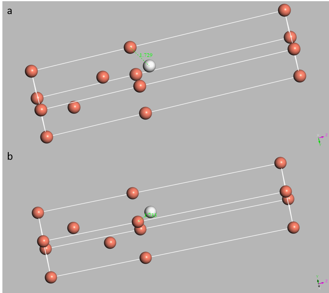
The crystal structure of Bi2Se3 is shown in Figure 1. The yellow atoms are Se atoms and the purple atoms are Bi atoms. Bi2Se3 has a rhombohedral structure of the space group D5 3d with R3m (#166). The lattice parameter are a=b=4.113 Å, c=28.5859 Å and the bond angle are a=b=90 degrees and c=120 degrees.

Figure 1, the crystal structure of Bi2Se3

2. Calculation of band structure without SOC

After the construction of the crystal, the geometry optimization is performed and the band structure is calculated, which is shown in Figure 3 and 4. As shown in these two figures, without considering SOC, the Bi2Se3 has a direct band gap, which is about 0.505 eV.

Figure 2. The structure of Bi2Se3 with the Brillouin zone (BZ). The blue lines show the Brillouin zone (the primitive unit cell of the reciprocal lattice) with the high symmetry points G (Center of the BZ), A (Center of a hexagonal face), H (Corner point), K (Middle of an edge joining two rectangular faces), M (Center of a rectangular face), L (Middle of an edge joining a hexagonal and a rectangular face).

Figure 3 The band structure of Bi2Se3 without SOC

Figure 4 The band structure (near G point) of Bi2Se3.

3. Calculation of band structure with SOC

The band structure with SOC is shown in Figure 5 and Figure 6. By including SOC, Bi2Se3 has an indirect band gap, which is about 0.281 eV. By comparing figures in Section 2 and Section 3, it can be seen that strong SOC has a significant impact on the band structure, and changes the band gap at the G point. Also since there is no direct band gap, it is possible that SOC induces the inversion between conduction and valence band at the G point, which could be a signal of a non-trivial topology.

Figure 5 The band structure of Bi2Se3 with SOC

Figure 6 The band structure of Bi2Se3 (near G point) with SOC

4.Calculation details

The pseudo atomic calculation performed for Bi: 6s2 6p3

The pseudo atomic calculation performed for Se: 3d10 4s2 4p4

Functional: GGA PBE

Cut off energy: 500eV

k-point set: 3*3*1

SCF tolerance: 1.0*10^ (-5) eV

Pseudopotential: Norm conserving

5. Conclusion and Discussion

In this project, the band structure of Bi2Se3 with and without SOC is calculated and compared. From the band structure, it can be seen that without changing other parameters, SOC can significantly change the band structure. So it is important to include SOC, especially for the elements with the atomic number being greater than the value of 50. Also by considering SOC, there is a signal of band inversion at G point in Bi2Se3, which could be an evidence of a non-trivial topology.

In this project, you can see that the parameters I choose are not very accurate. For one reason, I just want to point out the importance of spin-orbital coupling, so the accuracy of the results is not very high. For another reason, since the structure of Bi2Se3 are very complicated which needs huge calculation time and physical memory to calculate, it is impossible to improve the accuracy just using my computer.

For some future works, using the material studio, we can also get some other properties of Bulk Bi2Se3, such as the optical properties. Also, it is possible that we can build a slab with just a few layers to study the properties of the Bi2Se3 surface.


Hydrogen atoms adsorbed on Cu(111) surface

In this project, the absorption of H atom in the Cu (111) surface is analyzed and calculated. The H atom absorbed on Cu(111) can bind in two distinct threefold sites, the fcc sites and hcp sites shown in Figure 1. The energy difference between these two sites are calculated using Castep and the vibrational frequencies of H in each site is analyzed by calculating the elements of the Hessian matrix using finite-difference approximations. Then based on the vibrational frequencies, the zero-point energy can be obtained.

Figure 1. The absorption of H atom in the Cu (111) surface. the grey atoms are the H atoms and the red atoms are the Cu atoms. The H atoms are in the hcp sites (a) and fcc sites (b).

1. The slab model

As shown in Figure 1, an asymmetric slab model of 4 layers are used for the calculation. During the calculation, the two bottommost layers are fixed at bulk positions and all remaining atoms allowed to relax at z direction to obtain the optimized structures.

2. The optimized structures

For both two sites, the geometry optimization in the Castep is used to obtain the optimized structures, which are shown in Figure 2. We can also get the energy difference between these two structures. for hcp structure, the energy is -6738.743eV. For fcc structure, the energy is -6738.755eV. So the energy difference is 0.012eV. And since the energy of hcp structure is larger than the fcc structure, the fcc structure is more stable than the hcp structure.

Figure 2. The optimized structures for H atoms at the hcp sites (a) and fcc sites (b). The distances are 1.729 Ångstrom in a and 1.733 Ångstrom in b.

The calculation parameters for geometry optimization are listed here:
Atomic and pseudo atomic structure for H: 1s1
Atomic structure for Cu: 1s2 2s2 2p6 3s2 3p6 3d10 4s1
pseudo atomic structure for Cu: 3d10 4s1
Functional: GGA PBE
Cut off energy: 408.2eV
k-point set: 9*9*1
Energy convergence tolerance: 1.0e-005eV/atom
Force convergence tolerance: 0.03eV/Å
Stress convergence tolerance: 0.05GPa
Displacement convergence tolerance: 0.001Å

3. The vibrational frequencies

To obtain the vibrational frequencies, we need to get the Hessian matrix first. Using finite-difference approximations, the elements in the Hessian matrix can be obtained by the equation:

Table 1 shows the calculated energy and the Hessian matrix. Then the frequencies can be obtained by the equation:

λi is the eigenvalue of Hessian matrix. So we can get the frequencies shown in Table 2. The vibrational frequencies can be seen from the wave numbers of the vibrations. All the energy shown in these two table have 3  significant digits after the decimal place because we can already see the energy differences. All the Hessian matrix are shown in SI.

Table 1 The calculated energy and the Hessian matrix for hcp structure (a) and fcc structure (b).

Table 2 The eigenvalues of Hessian matrix, the vibrational frequencies and the zero-point energy for hcp structure (a) and fcc structure (b).

4. The zero-point energy correction

Since we have get the vibrational frequencies, the zero-point energy can be calculated by the equation E=∑(hv)/2.So as shown in Table 2, the total zero-point energy for hcp structure is 0.185eV and the total zero-point energy for fcc structure is 0.192eV. Then after considering the zero-point energy, the energy difference between fcc and hcp structures is 0.0046eV.

5. Conclusion and Discussion

In this project, the absorption of H atoms binding in two distinct threefold sites, the fcc sites and hcp sites on Cu (111) surface is calculated. Without considering the zero-point energy, the energy difference for these two structures is 0.012eV. With considering the zero-point energy, the energy difference for these two structures is 0.0046eV.

In this project, I assume that the H vibrations were uncoupled from the metal atoms in the surface and calculate the vibrational frequencies only moving the H atom. But this assumption is too simple and the vibrations should be more complicated in a real system. For example, we can consider the coupling between H atom and neighboring Cu atoms, which would be an interesting project for the future.

6. Reference

[1] S. J. Clark, M. D. Segall, C. J. Pickard, P. J. Hasnip, M. J. Probert, K. Refson, M. C. Payne, “First principles methods using CASTEP”, Zeitschrift fuer Kristallographie 220(5-6) pp. 567-570 (2005)

Determining the optimized geometry of water molecule

1. Introduction of the project

In this project, I calculated the optimized geometry of H2O. To get it, first, a cubic supercell (side length L angstroms) that is mostly empty space is built. Then the oxygen atom is placed in the supercell with fractional coordinates (0,0,0) and two hydrogen atoms are placed in the super cell with fractional coordinates (a/L, b/L,0) and (-a/L, b/L,0), shown in Figure 1. Next, by calculating the geometry optimization using CASTEP [1], the optimized geometry can be obtained, which includes the bond length and the bond angle.

Figure 1 The initial supercell structure. The red atoms are the oxygen atoms and the grey ones are hydrogen atoms.

During the calculation, the energy cutoff, the k point grid, the supercell lattice L can be changed to obtain most efficient and accurate results. The initial fractional coordinates of H can be changed to analyze if multiple initial geometries for each molecule converge to the same final state.

2. The parameters for the calculations

Some important parameters and inputs for the calculation are listed as following:
Atomic and pseudo atomic structure for H: 1s1
Atomic structure for O: 1s2 2s2 2p4
pseudo atomic structure for O: 2s2 2p4
Functional: GGA Perdew Burke Ernzerhof (PBA) functional
Pseudopotential: OTFG ultrasoft
The k points grid: investigated in the section 3
The energy cutoff: investigated in the section 4

3. The energy cut off

We can start with the k point grid of 3*3*3 and the supercell lattice L=10 Å. The initial fractional coordinates of H are chosen as (0.1, 0.05, 0) and (-0.1, 0.05, 0). From the calculation results shown in table 1, the energy cutoff can be chosen as 700eV.

Table 1 The calculation of the energy cut off.

4. The k point grid

We start with the energy cut off =700eV and the supercell lattice L=10 Å. The initial fractional coordinates of H are chosen as (0.1, 0.05, 0) and (-0.1, 0.05, 0). From the calculation results shown in table 2, the k point grid can be chosen as 1*1*1. It is easy to understand because the supercell is too large and we only consider the isolated molecule instead of the periodic system.

Table 2 The calculation results of the k point grid.

5. The supercell length L

Since we want to get the optimized geometry for an isolated molecule, the supercell lattice L need to be large enough to separate neighbouring molecules. As shown in the Table 3, the supercell length is varied, and the final supercell lengths, final bond length, bond angle are also changed. When initial supercell length is bigger than 10 Å, the final supercell lengths, final bond length and bond angle will become stable, which means the molecules are separated and they cannot feel the forces from neighbouring molecules. So we can choose the supercell length as 10 Å.

Table 3 The calculation results of the supercell length.

6. The initial hydrogen atom positions

The initial and final bond angle and bond length are changed as shown in Table     . As seen in table if we choose the initial bond angle equals 180°, the final bond angle will also be 180° . Because in this situation, the force along atoms direction is already balanced so the angle will not change. But if the initial bond angle is not 180°, the final bond length and angle are always 0.970 Å and around 104.5°.

Table 4 The calculation results for different initial hydrogen atom positions.

7. Conclusion

As shown in Figure 2, under the condition that the energy cut off is 700eV, the k points grid is 1*1*1, the supercell lattice length is 10Å, the initial bond length is 1.118 Å and the initial bond angle is 126.9°, the final results for bond length and angle are 0.970 Å and  104.582°. The experimental results for water molecule are: bond length is 0.958 Å bond angle is 104.45°. So the error for the bond length is about 1.2% and the error for the bond angle is about 0.1%.

Figure 2 The final water molecule structure for initial bond length is 1.118 Å and initial bond angle is 126.9°.

8. Discussion and future works

Although the results are very accurate with small errors, there are still some ways to further increase the accuracy. For example, during the calculation of geometry optimization, the parameters of convergence tolerance, such as Max. force, Max displacement, can be changed to increase the accuracy.

For some future works: Hydrogen bonding exists between water molecules, which will affect the water molecule structure, so it is worthwhile to try to calculate the Hydrogen bonding. Also since the water molecule has the dipole momentum, we can also calculate the dipole momentum of water molecules and compare it with the experimental results.

Reference

[1] S. J. Clark, M. D. Segall, C. J. Pickard, P. J. Hasnip, M. J. Probert, K. Refson, M. C. Payne, “First principles methods using CASTEP”, Zeitschrift fuer Kristallographie 220(5-6) pp. 567-570 (2005)

[2] The water molecule structure. https://www.worldofmolecules.com/solvents/water.htm

Determining the lattice constants for Hf

   For Project 1,  the lattice constants for Hf are calculated. Since Hf is an hcp metal with c/a=1.58, we need to calculate the energy by changing the lattice constant c while keeping c/a fixed. And the optimized a, c can be obtained by minimizing the free energy.

1. The hcp structure of Hf

   Figure 1 shows the unit cell of Hf hcp structure. OA, OB, OC are three lattice vectors. The lengths and angles of the lattices vectors (OA, OB, OC) are a, b, c and α, β, γ, respectively. To keep the symmetry, the constraints for the unit cell are a=b, α=β=90 degrees, γ=120 degrees.

Figure 1 The unit cell of Hf

2. The parameters for the calculations

Some important parameters and inputs for the calculation are listed as following:

Atomic structure for Hf:1s2 2s2 2p6 3s2 3p6 3d10 4s2 4p6 4d10 4f14 5s2 5p6 5d2 6s2

The core configuration of the pseudopotential: 1s2 2s2 2p6 3s2 3p6 3d10 4s2 4p6 4d10

Functional: GGA Perdew Burke Ernzerhof (PBA) functional

Pseudopotential: OTFG ultrasoft

Smearing width: 0.1

Origin shift of K points: 0, 0, 0

The k points grid: investigated in the next section

The energy cutoff: investigated in the next section

3. The convergence of the calculations

   Before starting the actual calculation for the lattice constant, it is important to explore the convergence of the calculations with respect to the number of k points and the energy cutoff. So the most accurate and efficient results can be obtained. For the following calculation, the lattice constant is fixed at c= 5.0511Å, a= 3.1946Å, while the size of k point grid and the energy cutoff are varied.

   (1) The number of k-points in the irreducible part of the BZ

     In this section 3.1, the energy cutoff is fixed at 400 eV, and the size of k point grid changes and Number of k-points in the irreducible part of the BZ (the number of k points) varies from 1 to 162, shown in Table 1. According to Table 1, the relations between Energy/atom, calculation time and the number of k points can be plotted, which are shown in Figure 2. As shown in Figure 2, the energy/atom becomes stable with the increase of k points. However, the calculation time also increases rapidly when the number of k points increases. By combining the results of these two graphs, 9*9*6 k points with 36 k points is chosen to obtain an accurate result with less calculation time.

   A little discussion here, since my calculation involves unit cells with different volumes, the k points need to be chosen so the density of k points in reciprocal space is comparable for the different supercells. But as shown in section 4, since the volumes of unit cell change just a little during the calculation, fixing the number of k points will not make much difference. So in section 4, the number of k points is chosen as 36 for all calculations.

Table 1 The calculation of different sizes of k point grid

Figure 2 The plots between Energy/atom, calculation time and the number of k points. The solid lines are just used for guide the eye.

(2) The energy cutoff

In this section, the number of k point is fixed at 36, and the energy cutoff varies from 200 to 800, shown in Table 2. And Figure 3 shows the relation between energy/atom, calculation time and energy cutoff. Although the energy/atom keeps increasing with the increase of energy cut off, the differences between each energy/atom are becoming smaller and smaller. On the other hand, the calculation time increases rapidly with the increase of energy cut off. In order to save the time and keep the accuracy, the energy cutoff is chosen as 435.4 eV.

Table 2 The calculation of different energy cutoff

Figure 3 The plots between energy/atom, calculation time and energy cutoff. The solid lines are used to guide the eye.

4 The calculation of the lattice constants

Using the results from section 3, the k points and the energy cutoff are chosen as 9*9*6 and 435.4 eV. Then lattice constants c and a are changed to obtain the minimum energy, shown in Table 3. As shown in Figure 4, the unit cell and the lattice constants can be predicted. As shown in Figure 4a, the quadratic relation between energy/atom and volume/atom only valid for a small range of lattice constants around the equilibrium value. A small range of volume/atom is chosen and the relation is re-plotted in Figure 4b. According to the fitting equation in Figure 4b, the fitting volume/atom is 22.64 Å^3 and the lattice constant are c=5.0673 Å, a=3.2072 Å. And for the experiment data, the lattice constants are a=3.1964 Å, c=5.0511 Å (1). So the calculation is accurate with an error of 0.3%.

Table 3 The calculation of energy with different lattice constants.

Figure 4 The plots between energy/atom and volume/atom. the solid lines are used to guide the eye. The dashed line is the fitting line.

5. Some discussion and future works

Although the calculation result is accurate with an error of 0.3%, there are still some ways to further increase the accuracy. First, the energy cut off can be increased so the energy/atom can be more precise. Second, we can calculate more points around the value c=5.05 Å and maybe a more accurate result can be obtained. Third, instead of using the quadratic fitting, we can use a higher order polynomial fitting.

For some future works: first, it is worthwhile changing the ratio c/a to determine the optimum value of c/a. Second, it should be interesting to analyze the behavior of energy at small or large lattice constants.

6. Reference:

(1) https://www.webelements.com/hafnium/crystal_structure.html